Model Explainers - For Classification

• TO DO:

• This will come after the lesson on converting regression task to classification

ADMIN: References

• REF: https://shap.readthedocs.io/en/latest/example_notebooks/tabular_examples/tree_based_models/NHANES I Survival Model.html

Lesson Objectives

By the end of this lesson students will be able to:

• Define a global vs local explanation

• Use the Shap package and interpret shap values.

Model Explainers

• There are packages with the sole purpose of better understanding how machine learning models make their predictions.

• Generally, model explainers will take the model and some of your data and apply some iterative process to try to quantify how the features are influencing the model’s output.

import pandas as pd
import numpy as np
import matplotlib as mpl
import matplotlib.pyplot as plt
import seaborn as sns
## Customization Options
# pd.set_option('display.float_format',lambda x: f"{x:,.4f}")
pd.set_option("display.max_columns",100)
plt.style.use(['fivethirtyeight','seaborn-talk'])
mpl.rcParams['figure.facecolor']='white'

## additional required imports
from sklearn.model_selection import train_test_split
from sklearn.preprocessing import OneHotEncoder, StandardScaler
from sklearn.impute import SimpleImputer
from sklearn.compose import make_column_transformer, make_column_selector, ColumnTransformer
from sklearn.pipeline import make_pipeline, Pipeline
from sklearn import metrics

from sklearn.base import clone

## fixing random for lesson generation
SEED = 321
np.random.seed(SEED)

## Adding folder above to path
import os, sys
sys.path.append(os.path.abspath('../../'))

## Load stack_functions with autoreload turned on
%load_ext autoreload
%autoreload 2
from CODE import stack_functions as sf
from CODE import prisoner_project_functions as pf

def show_code(function):
    import inspect 
    from IPython.display import display,Markdown, display_markdown
    code = inspect.getsource(function)
    md_txt = f"```python\n{code}\n```"
    return display(Markdown(md_txt))
    

# show_code(pf.evaluate_classification)

DATASET - NEED TO FINALIZE

Preprocessing Titanic

## Load in the King's County housing dataset and display the head and info
url = "https://docs.google.com/spreadsheets/d/e/2PACX-1vS6xDKNpWkBBdhZSqepy48bXo55QnRv1Xy6tXTKYzZLMPjZozMfYhHQjAcC8uj9hQ/pub?output=xlsx"

df = pd.read_excel(url,sheet_name='student-por')
# df.drop(columns=['G1','G2'])
df.info()
df.head()

<class 'pandas.core.frame.DataFrame'>
RangeIndex: 649 entries, 0 to 648
Data columns (total 33 columns):
 #   Column      Non-Null Count  Dtype  
---  ------      --------------  -----  
 0   school      649 non-null    object 
 1   sex         649 non-null    object 
 2   age         649 non-null    float64
 3   address     649 non-null    object 
 4   famsize     649 non-null    object 
 5   Pstatus     649 non-null    object 
 6   Medu        649 non-null    float64
 7   Fedu        649 non-null    float64
 8   Mjob        649 non-null    object 
 9   Fjob        649 non-null    object 
 10  reason      649 non-null    object 
 11  guardian    649 non-null    object 
 12  traveltime  649 non-null    float64
 13  studytime   649 non-null    float64
 14  failures    649 non-null    float64
 15  schoolsup   649 non-null    object 
 16  famsup      649 non-null    object 
 17  paid        649 non-null    object 
 18  activities  649 non-null    object 
 19  nursery     649 non-null    object 
 20  higher      649 non-null    object 
 21  internet    649 non-null    object 
 22  romantic    649 non-null    object 
 23  famrel      649 non-null    float64
 24  freetime    649 non-null    float64
 25  goout       649 non-null    float64
 26  Dalc        649 non-null    float64
 27  Walc        649 non-null    float64
 28  health      649 non-null    float64
 29  absences    649 non-null    float64
 30  G1          649 non-null    float64
 31  G2          649 non-null    float64
 32  G3          649 non-null    float64
dtypes: float64(16), object(17)
memory usage: 167.4+ KB

	school	sex	age	address	famsize	Pstatus	Medu	Fedu	Mjob	Fjob	reason	guardian	traveltime	studytime	failures	schoolsup	famsup	paid	activities	nursery	higher	internet	romantic	famrel	freetime	goout	Dalc	Walc	health	absences	G1	G2	G3
0	GP	F	18.0	U	GT3	A	4.0	4.0	at_home	teacher	course	mother	2.0	2.0	0.0	yes	no	no	no	yes	yes	no	no	4.0	3.0	4.0	1.0	1.0	3.0	4.0	0.0	11.0	11.0
1	GP	F	17.0	U	GT3	T	1.0	1.0	at_home	other	course	father	1.0	2.0	0.0	no	yes	no	no	no	yes	yes	no	5.0	3.0	3.0	1.0	1.0	3.0	2.0	9.0	11.0	11.0
2	GP	F	15.0	U	LE3	T	1.0	1.0	at_home	other	other	mother	1.0	2.0	0.0	yes	no	no	no	yes	yes	yes	no	4.0	3.0	2.0	2.0	3.0	3.0	6.0	12.0	13.0	12.0
3	GP	F	15.0	U	GT3	T	4.0	2.0	health	services	home	mother	1.0	3.0	0.0	no	yes	no	yes	yes	yes	yes	yes	3.0	2.0	2.0	1.0	1.0	5.0	0.0	14.0	14.0	14.0
4	GP	F	16.0	U	GT3	T	3.0	3.0	other	other	home	father	1.0	2.0	0.0	no	yes	no	no	yes	yes	no	no	4.0	3.0	2.0	1.0	2.0	5.0	0.0	11.0	13.0	13.0

QUICK CONVERT TO CLASS

• Maybe curve grades?

  • https://www.wikihow.com/Curve-Grades

• Or just make letter grades?

grade_cols = ['G1','G2','G3']
for col in grade_cols:
    df[f"{col}(%)"] = (df[col]/20) *100
# df[['G1%','G2%','G3%']]  = df[['G1','G2','G3']]/20*100
df

	school	sex	age	address	famsize	Pstatus	Medu	Fedu	Mjob	Fjob	reason	guardian	traveltime	studytime	failures	schoolsup	famsup	paid	activities	nursery	higher	internet	romantic	famrel	freetime	goout	Dalc	Walc	health	absences	G1	G2	G3	G1(%)	G2(%)	G3(%)
0	GP	F	18.0	U	GT3	A	4.0	4.0	at_home	teacher	course	mother	2.0	2.0	0.0	yes	no	no	no	yes	yes	no	no	4.0	3.0	4.0	1.0	1.0	3.0	4.0	0.0	11.0	11.0	0.0	55.0	55.0
1	GP	F	17.0	U	GT3	T	1.0	1.0	at_home	other	course	father	1.0	2.0	0.0	no	yes	no	no	no	yes	yes	no	5.0	3.0	3.0	1.0	1.0	3.0	2.0	9.0	11.0	11.0	45.0	55.0	55.0
2	GP	F	15.0	U	LE3	T	1.0	1.0	at_home	other	other	mother	1.0	2.0	0.0	yes	no	no	no	yes	yes	yes	no	4.0	3.0	2.0	2.0	3.0	3.0	6.0	12.0	13.0	12.0	60.0	65.0	60.0
3	GP	F	15.0	U	GT3	T	4.0	2.0	health	services	home	mother	1.0	3.0	0.0	no	yes	no	yes	yes	yes	yes	yes	3.0	2.0	2.0	1.0	1.0	5.0	0.0	14.0	14.0	14.0	70.0	70.0	70.0
4	GP	F	16.0	U	GT3	T	3.0	3.0	other	other	home	father	1.0	2.0	0.0	no	yes	no	no	yes	yes	no	no	4.0	3.0	2.0	1.0	2.0	5.0	0.0	11.0	13.0	13.0	55.0	65.0	65.0
...	...	...	...	...	...	...	...	...	...	...	...	...	...	...	...	...	...	...	...	...	...	...	...	...	...	...	...	...	...	...	...	...	...	...	...	...
644	MS	F	19.0	R	GT3	T	2.0	3.0	services	other	course	mother	1.0	3.0	1.0	no	no	no	yes	no	yes	yes	no	5.0	4.0	2.0	1.0	2.0	5.0	4.0	10.0	11.0	10.0	50.0	55.0	50.0
645	MS	F	18.0	U	LE3	T	3.0	1.0	teacher	services	course	mother	1.0	2.0	0.0	no	yes	no	no	yes	yes	yes	no	4.0	3.0	4.0	1.0	1.0	1.0	4.0	15.0	15.0	16.0	75.0	75.0	80.0
646	MS	F	18.0	U	GT3	T	1.0	1.0	other	other	course	mother	2.0	2.0	0.0	no	no	no	yes	yes	yes	no	no	1.0	1.0	1.0	1.0	1.0	5.0	6.0	11.0	12.0	9.0	55.0	60.0	45.0
647	MS	M	17.0	U	LE3	T	3.0	1.0	services	services	course	mother	2.0	1.0	0.0	no	no	no	no	no	yes	yes	no	2.0	4.0	5.0	3.0	4.0	2.0	6.0	10.0	10.0	10.0	50.0	50.0	50.0
648	MS	M	18.0	R	LE3	T	3.0	2.0	services	other	course	mother	3.0	1.0	0.0	no	no	no	no	no	yes	yes	no	4.0	4.0	1.0	3.0	4.0	5.0	4.0	10.0	11.0	11.0	50.0	55.0	55.0

649 rows × 36 columns

x = df['G3(%)'].values
x

array([55., 55., 60., 70., 65., 65., 65., 65., 85., 65., 70., 65., 60.,
       65., 75., 85., 70., 70., 35., 60., 70., 60., 70., 50., 50., 60.,
       60., 55., 65., 60., 55., 75., 75., 60., 60., 55., 70., 65., 60.,
       60., 50., 55., 75., 50., 55., 55., 65., 85., 65., 60., 65., 80.,
       45., 60., 65., 60., 75., 80., 70., 80., 80., 80., 50., 65., 60.,
       80., 60., 50., 55., 75., 55., 50., 55., 70., 55., 55., 55., 65.,
       50., 55., 60., 45., 55., 65., 60., 60., 55., 75., 55., 50., 55.,
       65., 60., 70., 60., 65., 55., 60., 65., 65., 40., 80., 60., 50.,
       80., 50., 50., 70., 55., 70., 70., 55., 50., 90., 50., 70., 80.,
       75., 55., 70., 70., 65., 65., 65., 55., 45., 55., 55., 75., 65.,
       60., 40., 55., 65., 60., 70., 55., 55., 55., 75., 50., 65., 60.,
       55., 55., 50., 50., 70., 45., 55., 45., 65., 55., 65., 55., 30.,
       60., 50., 55., 65., 55., 40., 55.,  0., 50., 65., 55., 65., 40.,
       50., 55., 55.,  5., 50., 45., 40., 50., 40., 40., 40., 55., 90.,
       65., 85., 50., 90., 50., 65., 75., 55., 70., 50., 55., 65., 55.,
       65., 85., 70., 80., 70., 55., 80., 70., 50., 65., 60., 60., 50.,
       60., 80., 70., 60., 80., 55., 75., 60., 75., 65., 65., 40., 60.,
       75., 65., 60., 60., 60., 65., 55., 55., 75., 50., 50., 65., 65.,
       55., 60., 70., 50., 80., 40., 85., 55., 55., 80., 60., 65., 65.,
       70., 45., 60., 80., 50., 65., 50., 50., 35., 40., 45., 75., 50.,
       55., 65., 40., 40., 50., 75., 70., 75., 60., 75., 75., 60., 75.,
       55., 50., 55., 80., 55., 65., 25., 50., 55., 35., 50., 30., 60.,
       65., 50., 65., 85., 55., 55., 70., 70., 65., 70., 80., 50., 60.,
       60., 75., 55., 60., 65., 65., 45., 80., 70., 60., 70., 50., 60.,
       80., 65., 90., 75., 80., 60., 50., 60., 65., 75., 50., 50., 55.,
       50., 65., 90., 65., 70., 70., 60., 90., 70., 75., 85., 80., 90.,
       95., 75., 75., 65., 70., 85., 85., 75., 65., 40., 80., 90., 55.,
       75., 55., 55., 75., 70., 85., 85., 75., 85., 70., 50., 65., 70.,
       85., 85., 65., 70., 55., 55., 45., 50., 65., 50., 85., 75., 70.,
       65., 85., 50., 65., 75., 55., 60., 50., 50., 75., 75., 60., 60.,
       70., 70., 75., 75., 80., 65., 85., 70., 70., 85., 85., 70., 65.,
       75., 80., 55., 65., 60., 60., 75., 85., 75., 85., 50., 75., 55.,
       90., 85., 70., 55., 85., 50., 65., 55., 60., 50., 55., 85., 45.,
       55., 55., 50., 35., 70., 55., 50., 40., 60., 60., 80.,  0., 45.,
       70., 40., 55., 45., 55., 45., 85., 65., 75., 55., 55., 40., 40.,
       45., 75., 55., 65., 50., 55., 70., 70., 60., 55., 40., 55., 70.,
       65., 65., 60., 60., 80., 50., 55., 70., 40., 55., 40., 50., 50.,
       55., 45., 55., 40., 55., 50., 50., 45., 50., 50., 45., 50., 50.,
       45., 65., 70., 50., 70., 80., 35., 65., 45., 70., 65., 55., 50.,
       50., 45., 90., 85., 50., 35., 40., 35., 50., 80., 75., 40.,  0.,
       40., 50., 40., 30., 40., 80., 70., 50., 45., 55., 45., 50., 40.,
       80., 60., 50., 70., 60., 55., 50., 55., 55., 60., 40., 60., 40.,
       80., 55., 55., 90., 65., 65., 50., 60., 50., 65., 55., 50., 50.,
       65., 50., 50., 60.,  0., 50., 45., 45.,  0., 45., 40., 40., 45.,
       35., 50., 50., 50., 55., 55., 50., 45., 50., 40., 35.,  0., 55.,
       40.,  0., 40., 45., 50., 35., 70., 65., 70., 90., 85., 90.,  0.,
       55., 70., 70., 50., 65.,  0., 50.,  0., 90., 60., 55., 60.,  0.,
       75., 55., 50., 60., 75., 70., 90., 75., 65., 75., 65., 45., 80.,
       45., 50.,  0., 50., 60., 45., 85., 60., 45., 70., 80., 45., 95.,
        0., 80.,  0.,  0., 75., 55., 50., 50., 80., 45., 50., 55.])

def calc_letter_grade(x):
    if isinstance(x,pd.Series):
        x = x.values
    letter_grades = {'A':x>=90,
                'B':(80<=x)&(x<90),
                'C':(70<=x)&(x<80),
                'D':(60<=x)&(x<70),
                'F':x<60}
    return np.select(letter_grades.values(), letter_grades.keys())

calc_letter_grade(df['G3(%)'])

array(['F', 'F', 'D', 'C', 'D', 'D', 'D', 'D', 'B', 'D', 'C', 'D', 'D',
       'D', 'C', 'B', 'C', 'C', 'F', 'D', 'C', 'D', 'C', 'F', 'F', 'D',
       'D', 'F', 'D', 'D', 'F', 'C', 'C', 'D', 'D', 'F', 'C', 'D', 'D',
       'D', 'F', 'F', 'C', 'F', 'F', 'F', 'D', 'B', 'D', 'D', 'D', 'B',
       'F', 'D', 'D', 'D', 'C', 'B', 'C', 'B', 'B', 'B', 'F', 'D', 'D',
       'B', 'D', 'F', 'F', 'C', 'F', 'F', 'F', 'C', 'F', 'F', 'F', 'D',
       'F', 'F', 'D', 'F', 'F', 'D', 'D', 'D', 'F', 'C', 'F', 'F', 'F',
       'D', 'D', 'C', 'D', 'D', 'F', 'D', 'D', 'D', 'F', 'B', 'D', 'F',
       'B', 'F', 'F', 'C', 'F', 'C', 'C', 'F', 'F', 'A', 'F', 'C', 'B',
       'C', 'F', 'C', 'C', 'D', 'D', 'D', 'F', 'F', 'F', 'F', 'C', 'D',
       'D', 'F', 'F', 'D', 'D', 'C', 'F', 'F', 'F', 'C', 'F', 'D', 'D',
       'F', 'F', 'F', 'F', 'C', 'F', 'F', 'F', 'D', 'F', 'D', 'F', 'F',
       'D', 'F', 'F', 'D', 'F', 'F', 'F', 'F', 'F', 'D', 'F', 'D', 'F',
       'F', 'F', 'F', 'F', 'F', 'F', 'F', 'F', 'F', 'F', 'F', 'F', 'A',
       'D', 'B', 'F', 'A', 'F', 'D', 'C', 'F', 'C', 'F', 'F', 'D', 'F',
       'D', 'B', 'C', 'B', 'C', 'F', 'B', 'C', 'F', 'D', 'D', 'D', 'F',
       'D', 'B', 'C', 'D', 'B', 'F', 'C', 'D', 'C', 'D', 'D', 'F', 'D',
       'C', 'D', 'D', 'D', 'D', 'D', 'F', 'F', 'C', 'F', 'F', 'D', 'D',
       'F', 'D', 'C', 'F', 'B', 'F', 'B', 'F', 'F', 'B', 'D', 'D', 'D',
       'C', 'F', 'D', 'B', 'F', 'D', 'F', 'F', 'F', 'F', 'F', 'C', 'F',
       'F', 'D', 'F', 'F', 'F', 'C', 'C', 'C', 'D', 'C', 'C', 'D', 'C',
       'F', 'F', 'F', 'B', 'F', 'D', 'F', 'F', 'F', 'F', 'F', 'F', 'D',
       'D', 'F', 'D', 'B', 'F', 'F', 'C', 'C', 'D', 'C', 'B', 'F', 'D',
       'D', 'C', 'F', 'D', 'D', 'D', 'F', 'B', 'C', 'D', 'C', 'F', 'D',
       'B', 'D', 'A', 'C', 'B', 'D', 'F', 'D', 'D', 'C', 'F', 'F', 'F',
       'F', 'D', 'A', 'D', 'C', 'C', 'D', 'A', 'C', 'C', 'B', 'B', 'A',
       'A', 'C', 'C', 'D', 'C', 'B', 'B', 'C', 'D', 'F', 'B', 'A', 'F',
       'C', 'F', 'F', 'C', 'C', 'B', 'B', 'C', 'B', 'C', 'F', 'D', 'C',
       'B', 'B', 'D', 'C', 'F', 'F', 'F', 'F', 'D', 'F', 'B', 'C', 'C',
       'D', 'B', 'F', 'D', 'C', 'F', 'D', 'F', 'F', 'C', 'C', 'D', 'D',
       'C', 'C', 'C', 'C', 'B', 'D', 'B', 'C', 'C', 'B', 'B', 'C', 'D',
       'C', 'B', 'F', 'D', 'D', 'D', 'C', 'B', 'C', 'B', 'F', 'C', 'F',
       'A', 'B', 'C', 'F', 'B', 'F', 'D', 'F', 'D', 'F', 'F', 'B', 'F',
       'F', 'F', 'F', 'F', 'C', 'F', 'F', 'F', 'D', 'D', 'B', 'F', 'F',
       'C', 'F', 'F', 'F', 'F', 'F', 'B', 'D', 'C', 'F', 'F', 'F', 'F',
       'F', 'C', 'F', 'D', 'F', 'F', 'C', 'C', 'D', 'F', 'F', 'F', 'C',
       'D', 'D', 'D', 'D', 'B', 'F', 'F', 'C', 'F', 'F', 'F', 'F', 'F',
       'F', 'F', 'F', 'F', 'F', 'F', 'F', 'F', 'F', 'F', 'F', 'F', 'F',
       'F', 'D', 'C', 'F', 'C', 'B', 'F', 'D', 'F', 'C', 'D', 'F', 'F',
       'F', 'F', 'A', 'B', 'F', 'F', 'F', 'F', 'F', 'B', 'C', 'F', 'F',
       'F', 'F', 'F', 'F', 'F', 'B', 'C', 'F', 'F', 'F', 'F', 'F', 'F',
       'B', 'D', 'F', 'C', 'D', 'F', 'F', 'F', 'F', 'D', 'F', 'D', 'F',
       'B', 'F', 'F', 'A', 'D', 'D', 'F', 'D', 'F', 'D', 'F', 'F', 'F',
       'D', 'F', 'F', 'D', 'F', 'F', 'F', 'F', 'F', 'F', 'F', 'F', 'F',
       'F', 'F', 'F', 'F', 'F', 'F', 'F', 'F', 'F', 'F', 'F', 'F', 'F',
       'F', 'F', 'F', 'F', 'F', 'F', 'C', 'D', 'C', 'A', 'B', 'A', 'F',
       'F', 'C', 'C', 'F', 'D', 'F', 'F', 'F', 'A', 'D', 'F', 'D', 'F',
       'C', 'F', 'F', 'D', 'C', 'C', 'A', 'C', 'D', 'C', 'D', 'F', 'B',
       'F', 'F', 'F', 'F', 'D', 'F', 'B', 'D', 'F', 'C', 'B', 'F', 'A',
       'F', 'B', 'F', 'F', 'C', 'F', 'F', 'F', 'B', 'F', 'F', 'F'],
      dtype='<U3')

# letter_grades = {'A':x>=90,
#                 'B':(80<=x)&(x<90),
#                 'C':(70<=x)&(x<80),
#                 'D':(60<=x)&(x<70),
#                 'F':x<60}
# np.select(letter_grades.values(), letter_grades.keys())

grade_cols_perc = [f"{col}(%)" for col in grade_cols]
df[grade_cols_perc]

	G1(%)	G2(%)	G3(%)
0	0.0	55.0	55.0
1	45.0	55.0	55.0
2	60.0	65.0	60.0
3	70.0	70.0	70.0
4	55.0	65.0	65.0
...	...	...	...
644	50.0	55.0	50.0
645	75.0	75.0	80.0
646	55.0	60.0	45.0
647	50.0	50.0	50.0
648	50.0	55.0	55.0

649 rows × 3 columns

for col in grade_cols_perc:
    df[col.replace("(%)",'_Class')] = calc_letter_grade(df[col])
df

	school	sex	age	address	famsize	Pstatus	Medu	Fedu	Mjob	Fjob	reason	guardian	traveltime	studytime	failures	schoolsup	famsup	paid	activities	nursery	higher	internet	romantic	famrel	freetime	goout	Dalc	Walc	health	absences	G1	G2	G3	G1(%)	G2(%)	G3(%)	G1_Class	G2_Class	G3_Class
0	GP	F	18.0	U	GT3	A	4.0	4.0	at_home	teacher	course	mother	2.0	2.0	0.0	yes	no	no	no	yes	yes	no	no	4.0	3.0	4.0	1.0	1.0	3.0	4.0	0.0	11.0	11.0	0.0	55.0	55.0	F	F	F
1	GP	F	17.0	U	GT3	T	1.0	1.0	at_home	other	course	father	1.0	2.0	0.0	no	yes	no	no	no	yes	yes	no	5.0	3.0	3.0	1.0	1.0	3.0	2.0	9.0	11.0	11.0	45.0	55.0	55.0	F	F	F
2	GP	F	15.0	U	LE3	T	1.0	1.0	at_home	other	other	mother	1.0	2.0	0.0	yes	no	no	no	yes	yes	yes	no	4.0	3.0	2.0	2.0	3.0	3.0	6.0	12.0	13.0	12.0	60.0	65.0	60.0	D	D	D
3	GP	F	15.0	U	GT3	T	4.0	2.0	health	services	home	mother	1.0	3.0	0.0	no	yes	no	yes	yes	yes	yes	yes	3.0	2.0	2.0	1.0	1.0	5.0	0.0	14.0	14.0	14.0	70.0	70.0	70.0	C	C	C
4	GP	F	16.0	U	GT3	T	3.0	3.0	other	other	home	father	1.0	2.0	0.0	no	yes	no	no	yes	yes	no	no	4.0	3.0	2.0	1.0	2.0	5.0	0.0	11.0	13.0	13.0	55.0	65.0	65.0	F	D	D
...	...	...	...	...	...	...	...	...	...	...	...	...	...	...	...	...	...	...	...	...	...	...	...	...	...	...	...	...	...	...	...	...	...	...	...	...	...	...	...
644	MS	F	19.0	R	GT3	T	2.0	3.0	services	other	course	mother	1.0	3.0	1.0	no	no	no	yes	no	yes	yes	no	5.0	4.0	2.0	1.0	2.0	5.0	4.0	10.0	11.0	10.0	50.0	55.0	50.0	F	F	F
645	MS	F	18.0	U	LE3	T	3.0	1.0	teacher	services	course	mother	1.0	2.0	0.0	no	yes	no	no	yes	yes	yes	no	4.0	3.0	4.0	1.0	1.0	1.0	4.0	15.0	15.0	16.0	75.0	75.0	80.0	C	C	B
646	MS	F	18.0	U	GT3	T	1.0	1.0	other	other	course	mother	2.0	2.0	0.0	no	no	no	yes	yes	yes	no	no	1.0	1.0	1.0	1.0	1.0	5.0	6.0	11.0	12.0	9.0	55.0	60.0	45.0	F	D	F
647	MS	M	17.0	U	LE3	T	3.0	1.0	services	services	course	mother	2.0	1.0	0.0	no	no	no	no	no	yes	yes	no	2.0	4.0	5.0	3.0	4.0	2.0	6.0	10.0	10.0	10.0	50.0	50.0	50.0	F	F	F
648	MS	M	18.0	R	LE3	T	3.0	2.0	services	other	course	mother	3.0	1.0	0.0	no	no	no	no	no	yes	yes	no	4.0	4.0	1.0	3.0	4.0	5.0	4.0	10.0	11.0	11.0	50.0	55.0	55.0	F	F	F

649 rows × 39 columns

fig, axes = plt.subplots(nrows=2,figsize=(8,8))
sns.histplot(data=df, x='G3(%)',ax=axes[0], binwidth=10)

sns.countplot(data=df,x='G3_Class',ax=axes[1],order=['F','D','C','B','A'])

<AxesSubplot:xlabel='G3_Class', ylabel='count'>

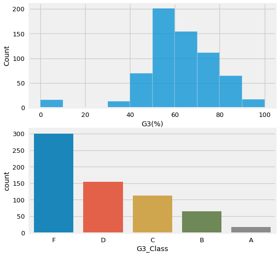
df['G3_Class'].value_counts()

F    301
D    154
C    112
B     65
A     17
Name: G3_Class, dtype: int64

## Define target as had a F or Above
df['target_F'] = df['G3_Class'] == 'F'
df['target_F'].value_counts()

False    348
True     301
Name: target_F, dtype: int64

g_cols = [c for c in df.columns if c.startswith("G")]
g_cols

['G1',
 'G2',
 'G3',
 'G1(%)',
 'G2(%)',
 'G3(%)',
 'G1_Class',
 'G2_Class',
 'G3_Class']

# ### Train Test Split
## Make x and y variables
drop_feats = [*g_cols]
y = df['target_F'].copy()
X = df.drop(columns=['target_F',*drop_feats]).copy()

## train-test-split with random state for reproducibility
X_train, X_test, y_train, y_test = train_test_split(X,y, random_state=SEED)


# ### Preprocessing + ColumnTransformer

## make categorical & numeric selectors
cat_sel = make_column_selector(dtype_include='object')
num_sel = make_column_selector(dtype_include='number')

## make pipelines for categorical vs numeric data
cat_pipe = make_pipeline(SimpleImputer(strategy='constant',
                                       fill_value='MISSING'),
                         OneHotEncoder(drop='if_binary', sparse=False))

num_pipe = make_pipeline(SimpleImputer(strategy='mean'))

## make the preprocessing column transformer
preprocessor = make_column_transformer((num_pipe, num_sel),
                                       (cat_pipe,cat_sel),
                                      verbose_feature_names_out=False)

## fit column transformer and run get_feature_names_out
preprocessor.fit(X_train)
feature_names = preprocessor.get_feature_names_out()

X_train_df = pd.DataFrame(preprocessor.transform(X_train), 
                          columns = feature_names, index = X_train.index)


X_test_df = pd.DataFrame(preprocessor.transform(X_test), 
                          columns = feature_names, index = X_test.index)
X_test_df.head(3)

	age	Medu	Fedu	traveltime	studytime	failures	famrel	freetime	goout	Dalc	Walc	health	absences	school_MS	sex_M	address_U	famsize_LE3	Pstatus_T	Mjob_at_home	Mjob_health	Mjob_other	Mjob_services	Mjob_teacher	Fjob_at_home	Fjob_health	Fjob_other	Fjob_services	Fjob_teacher	reason_course	reason_home	reason_other	reason_reputation	guardian_father	guardian_mother	guardian_other	schoolsup_yes	famsup_yes	paid_yes	activities_yes	nursery_yes	higher_yes	internet_yes	romantic_yes
104	15.0	3.0	4.0	1.0	2.0	0.0	5.0	4.0	4.0	1.0	1.0	1.0	0.0	0.0	1.0	1.0	0.0	0.0	0.0	0.0	0.0	1.0	0.0	0.0	0.0	1.0	0.0	0.0	1.0	0.0	0.0	0.0	0.0	1.0	0.0	0.0	1.0	0.0	1.0	1.0	1.0	1.0	0.0
284	18.0	2.0	1.0	1.0	1.0	2.0	3.0	2.0	5.0	2.0	5.0	5.0	4.0	0.0	1.0	1.0	0.0	1.0	0.0	0.0	0.0	1.0	0.0	0.0	0.0	0.0	1.0	0.0	0.0	0.0	1.0	0.0	0.0	1.0	0.0	0.0	0.0	0.0	0.0	0.0	0.0	1.0	0.0
579	18.0	1.0	3.0	1.0	1.0	0.0	4.0	3.0	3.0	2.0	3.0	3.0	0.0	1.0	1.0	1.0	1.0	1.0	1.0	0.0	0.0	0.0	0.0	0.0	0.0	0.0	1.0	0.0	1.0	0.0	0.0	0.0	0.0	1.0	0.0	0.0	0.0	0.0	0.0	1.0	0.0	1.0	1.0

## fit random fores
from sklearn.ensemble import RandomForestClassifier
rf_clf = RandomForestClassifier()
rf_clf.fit(X_train_df,y_train)
sf.evaluate_classification(rf_clf,X_test_df,y_test, 
                       X_train=X_train_df, y_train=y_train)#linreg(rf_reg,X_train_zips,y_train,X_test_zips,y_test)

------------------------------------------------------------
	CLASSIFICATION REPORT - Test Data
------------------------------------------------------------
              precision    recall  f1-score   support

       False       0.78      0.85      0.82        88
        True       0.81      0.72      0.76        75

    accuracy                           0.79       163
   macro avg       0.79      0.79      0.79       163
weighted avg       0.79      0.79      0.79       163

/opt/homebrew/Caskroom/miniforge/base/envs/dojo-env/lib/python3.8/site-packages/sklearn/utils/deprecation.py:87: FutureWarning: Function plot_roc_curve is deprecated; Function :func:`plot_roc_curve` is deprecated in 1.0 and will be removed in 1.2. Use one of the class methods: :meth:`sklearn.metric.RocCurveDisplay.from_predictions` or :meth:`sklearn.metric.RocCurveDisplay.from_estimator`.
  warnings.warn(msg, category=FutureWarning)

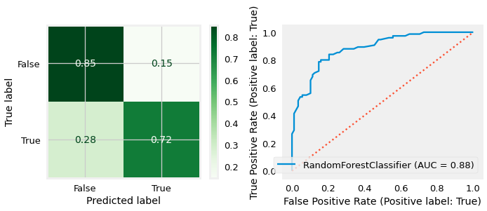
Training Score = 1.00
Test Score = 0.79

Loading Joblib of Regressions from Lesson 04

# import joblib
# ## If showing joblib in prior lesson, this cell will be included and further explained
# loaded_data = joblib.load("../4_Feature_Importance/lesson_04.joblib")
# loaded_data.keys()

# ## If showing joblib in prior lesson, this cell will be included and further explained
# X_train_reg = loaded_data['X_train'].copy()
# y_train_reg = loaded_data['y_train'].copy()
# X_test_df_reg = loaded_data['X_test'].copy()
# y_test_reg = loaded_data['y_test'].copy()
# lin_reg = loaded_data['lin_reg']
# rf_reg = loaded_data['rf_reg']

Using SHAP for Model Interpretation

• SHAP (SHapley Additive exPlanations))

  • Repository

  • Documentation

• SHAP uses game theory to calcualte Shapely values for each feature in the dataset.

• Shapely values are calculated by iteratively testing each feature’s contribution to the model by comparing the model’s performance with vs. without the feature. (The “marginal contribution” of the feature to the model’s performance).

Papers, Book Excerpts, and Blogs

• White Paper on Shapely Values

• Intepretable Machine Learning Book - Section on SHAP

• Towards Data Science Blog Posts:

  • Explain Your Model with SHAP Values

  • Explain Any Model with SHAP KernelExplaibner

Videos/Talks:

• Explaining Machine Learning Models (in general).

  • “Open the Black Box: an intro to Model Interpretability with LIME and SHAP

• Understanding Shapely/SHAP Values:

  • AI Simplified: SHAP Values in Machine Learning - (Intuitive Explanation)

  • Explainable AI explained! | #4 SHAP - (Math Calculation Explanation)

How To Use Shap

• Import and initialize javascript:

import shap 
shap.initjs()

import shap
shap.initjs()

Shap Explainers

• shap has several types of model explainers that are optimized for different types of models.

Explainers and their use cases:

Explainer	Description
shap.Explainer	Uses Shapley values to explain any machine learning model or python function.
shap.explainers.Tree	Uses Tree SHAP algorithms to explain the output of ensemble tree models.
shap.explainers.Linear	Computes SHAP values for a linear model, optionally accounting for inter-feature correlations.
shap.explainers.Permutation	This method approximates the Shapley values by iterating through permutations of the inputs.
shap.explainers.Sampling	This is an extension of the Shapley sampling values explanation method (aka.
shap.explainers.Additive	Computes SHAP values for generalized additive models.
shap.explainers.other.Coefficent	Simply returns the model coefficents as the feature attributions.
shap.explainers.other.Random	Simply returns random (normally distributed) feature attributions.
shap.explainers.other.LimeTabular	Simply wrap of lime.lime_tabular.LimeTabularExplainer into the common shap interface.
shap.explainers.other.Maple	Simply wraps MAPLE into the common SHAP interface.
shap.explainers.other.TreeMaple	Simply tree MAPLE into the common SHAP interface.
shap.explainers.other.TreeGain	Simply returns the global gain/gini feature importances for tree models.

• See this blog post for intro to topic and how to use with trees

• For non-tree/random forest models see this follow up post

Preparing Data for Shap

• Shap’s approach to explaining models can be very resource-intensive for complex models such as our RandomForest.

• To get around this issue, shap includes a convenient smapling function to save a small sample from one of our X variables.

X_shap = shap.sample(X_train_df,nsamples=200,random_state=321)
X_shap

	age	Medu	Fedu	traveltime	studytime	failures	famrel	freetime	goout	Dalc	Walc	health	absences	school_MS	sex_M	address_U	famsize_LE3	Pstatus_T	Mjob_at_home	Mjob_health	Mjob_other	Mjob_services	Mjob_teacher	Fjob_at_home	Fjob_health	Fjob_other	Fjob_services	Fjob_teacher	reason_course	reason_home	reason_other	reason_reputation	guardian_father	guardian_mother	guardian_other	schoolsup_yes	famsup_yes	paid_yes	activities_yes	nursery_yes	higher_yes	internet_yes	romantic_yes
473	16.0	2.0	1.0	2.0	1.0	0.0	2.0	4.0	3.0	2.0	3.0	4.0	4.0	1.0	1.0	1.0	1.0	1.0	1.0	0.0	0.0	0.0	0.0	0.0	0.0	0.0	1.0	0.0	1.0	0.0	0.0	0.0	0.0	1.0	0.0	0.0	1.0	0.0	1.0	1.0	1.0	1.0	0.0
340	17.0	3.0	3.0	1.0	1.0	0.0	4.0	4.0	3.0	1.0	3.0	5.0	0.0	0.0	1.0	1.0	0.0	1.0	0.0	1.0	0.0	0.0	0.0	0.0	0.0	1.0	0.0	0.0	0.0	1.0	0.0	0.0	0.0	1.0	0.0	0.0	1.0	0.0	0.0	1.0	1.0	1.0	0.0
452	16.0	2.0	2.0	3.0	2.0	0.0	4.0	4.0	5.0	1.0	1.0	4.0	4.0	1.0	0.0	0.0	0.0	1.0	0.0	0.0	1.0	0.0	0.0	0.0	0.0	1.0	0.0	0.0	1.0	0.0	0.0	0.0	0.0	1.0	0.0	0.0	1.0	0.0	0.0	1.0	1.0	1.0	0.0
555	16.0	1.0	2.0	1.0	3.0	0.0	4.0	3.0	4.0	1.0	1.0	3.0	5.0	1.0	0.0	0.0	0.0	1.0	0.0	0.0	1.0	0.0	0.0	0.0	0.0	1.0	0.0	0.0	0.0	1.0	0.0	0.0	1.0	0.0	0.0	1.0	1.0	0.0	0.0	0.0	1.0	1.0	1.0
70	16.0	3.0	1.0	2.0	4.0	0.0	4.0	3.0	2.0	1.0	1.0	5.0	2.0	0.0	1.0	1.0	0.0	1.0	0.0	0.0	1.0	0.0	0.0	0.0	0.0	1.0	0.0	0.0	0.0	0.0	0.0	1.0	1.0	0.0	0.0	0.0	1.0	0.0	0.0	1.0	1.0	1.0	0.0
...	...	...	...	...	...	...	...	...	...	...	...	...	...	...	...	...	...	...	...	...	...	...	...	...	...	...	...	...	...	...	...	...	...	...	...	...	...	...	...	...	...	...	...
353	18.0	1.0	4.0	1.0	2.0	0.0	3.0	4.0	4.0	1.0	2.0	5.0	2.0	0.0	0.0	1.0	0.0	1.0	0.0	0.0	1.0	0.0	0.0	0.0	0.0	0.0	0.0	1.0	0.0	1.0	0.0	0.0	0.0	1.0	0.0	1.0	1.0	0.0	0.0	0.0	1.0	0.0	1.0
443	15.0	4.0	1.0	1.0	2.0	0.0	5.0	3.0	4.0	1.0	2.0	2.0	7.0	1.0	1.0	0.0	1.0	1.0	0.0	1.0	0.0	0.0	0.0	0.0	0.0	0.0	1.0	0.0	0.0	0.0	0.0	1.0	1.0	0.0	0.0	0.0	1.0	0.0	1.0	1.0	1.0	1.0	0.0
120	15.0	1.0	2.0	1.0	2.0	0.0	3.0	2.0	3.0	1.0	2.0	1.0	0.0	0.0	0.0	1.0	0.0	1.0	1.0	0.0	0.0	0.0	0.0	0.0	0.0	0.0	1.0	0.0	1.0	0.0	0.0	0.0	0.0	1.0	0.0	0.0	0.0	0.0	0.0	0.0	1.0	1.0	0.0
294	18.0	2.0	2.0	1.0	2.0	0.0	3.0	2.0	3.0	1.0	1.0	5.0	4.0	0.0	0.0	0.0	0.0	1.0	0.0	0.0	1.0	0.0	0.0	0.0	0.0	1.0	0.0	0.0	0.0	1.0	0.0	0.0	0.0	1.0	0.0	1.0	0.0	0.0	0.0	1.0	1.0	0.0	0.0
340	17.0	3.0	3.0	1.0	1.0	0.0	4.0	4.0	3.0	1.0	3.0	5.0	0.0	0.0	1.0	1.0	0.0	1.0	0.0	1.0	0.0	0.0	0.0	0.0	0.0	1.0	0.0	0.0	0.0	1.0	0.0	0.0	0.0	1.0	0.0	0.0	1.0	0.0	0.0	1.0	1.0	1.0	0.0

200 rows × 43 columns

## get the corresponding y-values
y_shap = y_train.loc[X_shap.index]
y_shap

473     True
340    False
452     True
555    False
70      True
       ...  
353     True
443     True
120    False
294    False
340    False
Name: target_F, Length: 200, dtype: bool

Explaining Our RandomForest

1. Create a shap explainer using your fit model.

explainer = shap.TreeExplainer(rf_reg)

1. Get shapely values from explainer for your training data

shap_values = explainer(X_shap)

1. Select which type of the available plots you’d like to visualize

• Types of Plots:

  • summary_plot()

  • dependence_plot()

  • force_plot() for a given observation

  • force_plot() for all data

# # TEMP
# X_shap = shap.sample(X_train_df,nsamples=200,random_state=321)

# explainer = shap.TreeExplainer(rf_reg)
# shap_values_demo = explainer.shap_values(X_shap,y_shap)
# shap_values_demo[1]

X_train_df

	age	Medu	Fedu	traveltime	studytime	failures	famrel	freetime	goout	Dalc	Walc	health	absences	school_MS	sex_M	address_U	famsize_LE3	Pstatus_T	Mjob_at_home	Mjob_health	Mjob_other	Mjob_services	Mjob_teacher	Fjob_at_home	Fjob_health	Fjob_other	Fjob_services	Fjob_teacher	reason_course	reason_home	reason_other	reason_reputation	guardian_father	guardian_mother	guardian_other	schoolsup_yes	famsup_yes	paid_yes	activities_yes	nursery_yes	higher_yes	internet_yes	romantic_yes
54	15.0	3.0	3.0	1.0	1.0	0.0	5.0	3.0	4.0	4.0	4.0	1.0	0.0	0.0	0.0	1.0	1.0	0.0	0.0	0.0	1.0	0.0	0.0	0.0	0.0	1.0	0.0	0.0	0.0	0.0	1.0	0.0	0.0	1.0	0.0	0.0	0.0	0.0	0.0	1.0	1.0	1.0	0.0
208	16.0	2.0	3.0	2.0	1.0	0.0	5.0	3.0	3.0	1.0	1.0	3.0	0.0	0.0	1.0	1.0	0.0	1.0	0.0	0.0	1.0	0.0	0.0	0.0	0.0	1.0	0.0	0.0	0.0	1.0	0.0	0.0	1.0	0.0	0.0	0.0	0.0	0.0	0.0	1.0	1.0	1.0	0.0
23	16.0	2.0	2.0	2.0	2.0	0.0	5.0	4.0	4.0	2.0	4.0	5.0	2.0	0.0	1.0	1.0	1.0	1.0	0.0	0.0	1.0	0.0	0.0	0.0	0.0	1.0	0.0	0.0	0.0	0.0	0.0	1.0	0.0	1.0	0.0	0.0	1.0	0.0	1.0	1.0	1.0	1.0	0.0
547	16.0	4.0	1.0	1.0	1.0	0.0	4.0	1.0	2.0	2.0	1.0	2.0	0.0	1.0	1.0	0.0	1.0	1.0	0.0	0.0	1.0	0.0	0.0	1.0	0.0	0.0	0.0	0.0	0.0	0.0	1.0	0.0	1.0	0.0	0.0	0.0	0.0	0.0	0.0	1.0	1.0	1.0	0.0
604	18.0	1.0	1.0	3.0	2.0	1.0	4.0	4.0	2.0	1.0	2.0	2.0	2.0	1.0	0.0	1.0	0.0	1.0	1.0	0.0	0.0	0.0	0.0	0.0	0.0	0.0	1.0	0.0	1.0	0.0	0.0	0.0	0.0	1.0	0.0	0.0	0.0	0.0	0.0	1.0	0.0	0.0	0.0
...	...	...	...	...	...	...	...	...	...	...	...	...	...	...	...	...	...	...	...	...	...	...	...	...	...	...	...	...	...	...	...	...	...	...	...	...	...	...	...	...	...	...	...
410	17.0	2.0	2.0	1.0	2.0	0.0	4.0	3.0	4.0	1.0	3.0	4.0	0.0	0.0	0.0	1.0	0.0	1.0	0.0	0.0	0.0	1.0	0.0	0.0	0.0	0.0	1.0	0.0	0.0	0.0	0.0	1.0	0.0	1.0	0.0	0.0	1.0	0.0	1.0	1.0	1.0	1.0	0.0
168	15.0	2.0	3.0	1.0	2.0	0.0	4.0	4.0	4.0	1.0	1.0	1.0	0.0	0.0	1.0	0.0	0.0	1.0	1.0	0.0	0.0	0.0	0.0	0.0	0.0	0.0	1.0	0.0	1.0	0.0	0.0	0.0	0.0	1.0	0.0	1.0	0.0	1.0	1.0	1.0	1.0	0.0	0.0
401	18.0	4.0	3.0	1.0	3.0	0.0	5.0	4.0	5.0	2.0	3.0	5.0	0.0	0.0	1.0	1.0	0.0	1.0	0.0	0.0	0.0	0.0	1.0	0.0	0.0	1.0	0.0	0.0	1.0	0.0	0.0	0.0	0.0	1.0	0.0	0.0	1.0	0.0	0.0	1.0	1.0	1.0	1.0
124	16.0	2.0	2.0	1.0	2.0	0.0	5.0	4.0	4.0	1.0	1.0	5.0	0.0	0.0	0.0	1.0	0.0	1.0	0.0	0.0	1.0	0.0	0.0	0.0	0.0	1.0	0.0	0.0	0.0	1.0	0.0	0.0	0.0	1.0	0.0	0.0	0.0	0.0	0.0	1.0	1.0	1.0	1.0
538	16.0	2.0	2.0	1.0	3.0	0.0	4.0	3.0	3.0	2.0	2.0	5.0	2.0	1.0	0.0	0.0	1.0	1.0	0.0	0.0	1.0	0.0	0.0	0.0	0.0	1.0	0.0	0.0	1.0	0.0	0.0	0.0	0.0	1.0	0.0	0.0	1.0	0.0	0.0	0.0	1.0	0.0	1.0

486 rows × 43 columns

# X_shap = shap.sample(X_train_df,nsamples=200,random_state=SEED)
X_shap = X_train_df.copy()
explainer = shap.TreeExplainer(rf_clf)
shap_values = explainer(X_shap,y_shap)
shap_values[0]

.values =
array([[ 0.008814  , -0.008814  ],
       [ 0.01795532, -0.01795532],
       [ 0.02879442, -0.02879442],
       [ 0.01450603, -0.01450603],
       [-0.0252331 ,  0.0252331 ],
       [ 0.03957148, -0.03957148],
       [ 0.01838909, -0.01838909],
       [ 0.01160811, -0.01160811],
       [ 0.00272609, -0.00272609],
       [-0.05268544,  0.05268544],
       [-0.03223627,  0.03223627],
       [ 0.03554543, -0.03554543],
       [ 0.04377185, -0.04377185],
       [ 0.04092553, -0.04092553],
       [ 0.03401933, -0.03401933],
       [ 0.0091445 , -0.0091445 ],
       [ 0.00462221, -0.00462221],
       [-0.00037379,  0.00037379],
       [ 0.02386322, -0.02386322],
       [ 0.0028716 , -0.0028716 ],
       [ 0.01790442, -0.01790442],
       [ 0.00170321, -0.00170321],
       [-0.00017733,  0.00017733],
       [ 0.00139468, -0.00139468],
       [ 0.00167475, -0.00167475],
       [ 0.0046005 , -0.0046005 ],
       [ 0.0026676 , -0.0026676 ],
       [-0.00230831,  0.00230831],
       [ 0.01803168, -0.01803168],
       [-0.00099782,  0.00099782],
       [ 0.00110679, -0.00110679],
       [ 0.00204202, -0.00204202],
       [ 0.00107499, -0.00107499],
       [-0.00057534,  0.00057534],
       [-0.00089219,  0.00089219],
       [ 0.00570406, -0.00570406],
       [ 0.00939121, -0.00939121],
       [ 0.00087085, -0.00087085],
       [-0.00290892,  0.00290892],
       [-0.00238875,  0.00238875],
       [ 0.02169016, -0.02169016],
       [ 0.01027966, -0.01027966],
       [ 0.00678408, -0.00678408]])

.base_values =
array([0.5367284, 0.4632716])

.data =
array([15.,  3.,  3.,  1.,  1.,  0.,  5.,  3.,  4.,  4.,  4.,  1.,  0.,
        0.,  0.,  1.,  1.,  0.,  0.,  0.,  1.,  0.,  0.,  0.,  0.,  1.,
        0.,  0.,  0.,  0.,  1.,  0.,  0.,  1.,  0.,  0.,  0.,  0.,  0.,
        1.,  1.,  1.,  0.])

X_shap.shape

(486, 43)

shap_values.shape

(486, 43, 2)

• We can see that shap calculated values for every row/column in our X_shap variable.

• What does the first row’s shap values look like?

shap_values[0]

.values =
array([[ 0.008814  , -0.008814  ],
       [ 0.01795532, -0.01795532],
       [ 0.02879442, -0.02879442],
       [ 0.01450603, -0.01450603],
       [-0.0252331 ,  0.0252331 ],
       [ 0.03957148, -0.03957148],
       [ 0.01838909, -0.01838909],
       [ 0.01160811, -0.01160811],
       [ 0.00272609, -0.00272609],
       [-0.05268544,  0.05268544],
       [-0.03223627,  0.03223627],
       [ 0.03554543, -0.03554543],
       [ 0.04377185, -0.04377185],
       [ 0.04092553, -0.04092553],
       [ 0.03401933, -0.03401933],
       [ 0.0091445 , -0.0091445 ],
       [ 0.00462221, -0.00462221],
       [-0.00037379,  0.00037379],
       [ 0.02386322, -0.02386322],
       [ 0.0028716 , -0.0028716 ],
       [ 0.01790442, -0.01790442],
       [ 0.00170321, -0.00170321],
       [-0.00017733,  0.00017733],
       [ 0.00139468, -0.00139468],
       [ 0.00167475, -0.00167475],
       [ 0.0046005 , -0.0046005 ],
       [ 0.0026676 , -0.0026676 ],
       [-0.00230831,  0.00230831],
       [ 0.01803168, -0.01803168],
       [-0.00099782,  0.00099782],
       [ 0.00110679, -0.00110679],
       [ 0.00204202, -0.00204202],
       [ 0.00107499, -0.00107499],
       [-0.00057534,  0.00057534],
       [-0.00089219,  0.00089219],
       [ 0.00570406, -0.00570406],
       [ 0.00939121, -0.00939121],
       [ 0.00087085, -0.00087085],
       [-0.00290892,  0.00290892],
       [-0.00238875,  0.00238875],
       [ 0.02169016, -0.02169016],
       [ 0.01027966, -0.01027966],
       [ 0.00678408, -0.00678408]])

.base_values =
array([0.5367284, 0.4632716])

.data =
array([15.,  3.,  3.,  1.,  1.,  0.,  5.,  3.,  4.,  4.,  4.,  1.,  0.,
        0.,  0.,  1.,  1.,  0.,  0.,  0.,  1.,  0.,  0.,  0.,  0.,  1.,
        0.,  0.,  0.,  0.,  1.,  0.,  0.,  1.,  0.,  0.,  0.,  0.,  0.,
        1.,  1.,  1.,  0.])

• Notice above that we do not seem to have a simple numpy array.

type(shap_values[0])

shap._explanation.Explanation

explanation_0 = shap_values[0]
explanation_0

.values =
array([[ 0.008814  , -0.008814  ],
       [ 0.01795532, -0.01795532],
       [ 0.02879442, -0.02879442],
       [ 0.01450603, -0.01450603],
       [-0.0252331 ,  0.0252331 ],
       [ 0.03957148, -0.03957148],
       [ 0.01838909, -0.01838909],
       [ 0.01160811, -0.01160811],
       [ 0.00272609, -0.00272609],
       [-0.05268544,  0.05268544],
       [-0.03223627,  0.03223627],
       [ 0.03554543, -0.03554543],
       [ 0.04377185, -0.04377185],
       [ 0.04092553, -0.04092553],
       [ 0.03401933, -0.03401933],
       [ 0.0091445 , -0.0091445 ],
       [ 0.00462221, -0.00462221],
       [-0.00037379,  0.00037379],
       [ 0.02386322, -0.02386322],
       [ 0.0028716 , -0.0028716 ],
       [ 0.01790442, -0.01790442],
       [ 0.00170321, -0.00170321],
       [-0.00017733,  0.00017733],
       [ 0.00139468, -0.00139468],
       [ 0.00167475, -0.00167475],
       [ 0.0046005 , -0.0046005 ],
       [ 0.0026676 , -0.0026676 ],
       [-0.00230831,  0.00230831],
       [ 0.01803168, -0.01803168],
       [-0.00099782,  0.00099782],
       [ 0.00110679, -0.00110679],
       [ 0.00204202, -0.00204202],
       [ 0.00107499, -0.00107499],
       [-0.00057534,  0.00057534],
       [-0.00089219,  0.00089219],
       [ 0.00570406, -0.00570406],
       [ 0.00939121, -0.00939121],
       [ 0.00087085, -0.00087085],
       [-0.00290892,  0.00290892],
       [-0.00238875,  0.00238875],
       [ 0.02169016, -0.02169016],
       [ 0.01027966, -0.01027966],
       [ 0.00678408, -0.00678408]])

.base_values =
array([0.5367284, 0.4632716])

.data =
array([15.,  3.,  3.,  1.,  1.,  0.,  5.,  3.,  4.,  4.,  4.,  1.,  0.,
        0.,  0.,  1.,  1.,  0.,  0.,  0.,  1.,  0.,  0.,  0.,  0.,  1.,
        0.,  0.,  0.,  0.,  1.,  0.,  0.,  1.,  0.,  0.,  0.,  0.,  0.,
        1.,  1.,  1.,  0.])

• Each entry in the shap_values array is new type of object called an Explanation.

  • Each Explanation has:

    • values:the shap values calculated for this observation/row.

      • For classification models, there is a column with values for each target.

    • base_values: the final shap output value

    • data: the original input feature

## Showing .data is the same as the raw X_shap
explanation_0.data

array([15.,  3.,  3.,  1.,  1.,  0.,  5.,  3.,  4.,  4.,  4.,  1.,  0.,
        0.,  0.,  1.,  1.,  0.,  0.,  0.,  1.,  0.,  0.,  0.,  0.,  1.,
        0.,  0.,  0.,  0.,  1.,  0.,  0.,  1.,  0.,  0.,  0.,  0.,  0.,
        1.,  1.,  1.,  0.])

X_shap.iloc[0].values

array([15.,  3.,  3.,  1.,  1.,  0.,  5.,  3.,  4.,  4.,  4.,  1.,  0.,
        0.,  0.,  1.,  1.,  0.,  0.,  0.,  1.,  0.,  0.,  0.,  0.,  1.,
        0.,  0.,  0.,  0.,  1.,  0.,  0.,  1.,  0.,  0.,  0.,  0.,  0.,
        1.,  1.,  1.,  0.])

## showing the .values
pd.DataFrame(explanation_0.values,index=X_shap.columns)

	0	1
age	0.008814	-0.008814
Medu	0.017955	-0.017955
Fedu	0.028794	-0.028794
traveltime	0.014506	-0.014506
studytime	-0.025233	0.025233
failures	0.039571	-0.039571
famrel	0.018389	-0.018389
freetime	0.011608	-0.011608
goout	0.002726	-0.002726
Dalc	-0.052685	0.052685
Walc	-0.032236	0.032236
health	0.035545	-0.035545
absences	0.043772	-0.043772
school_MS	0.040926	-0.040926
sex_M	0.034019	-0.034019
address_U	0.009145	-0.009145
famsize_LE3	0.004622	-0.004622
Pstatus_T	-0.000374	0.000374
Mjob_at_home	0.023863	-0.023863
Mjob_health	0.002872	-0.002872
Mjob_other	0.017904	-0.017904
Mjob_services	0.001703	-0.001703
Mjob_teacher	-0.000177	0.000177
Fjob_at_home	0.001395	-0.001395
Fjob_health	0.001675	-0.001675
Fjob_other	0.004601	-0.004601
Fjob_services	0.002668	-0.002668
Fjob_teacher	-0.002308	0.002308
reason_course	0.018032	-0.018032
reason_home	-0.000998	0.000998
reason_other	0.001107	-0.001107
reason_reputation	0.002042	-0.002042
guardian_father	0.001075	-0.001075
guardian_mother	-0.000575	0.000575
guardian_other	-0.000892	0.000892
schoolsup_yes	0.005704	-0.005704
famsup_yes	0.009391	-0.009391
paid_yes	0.000871	-0.000871
activities_yes	-0.002909	0.002909
nursery_yes	-0.002389	0.002389
higher_yes	0.021690	-0.021690
internet_yes	0.010280	-0.010280
romantic_yes	0.006784	-0.006784

📌 BOOKMARK

Shap Visualizations - Classification

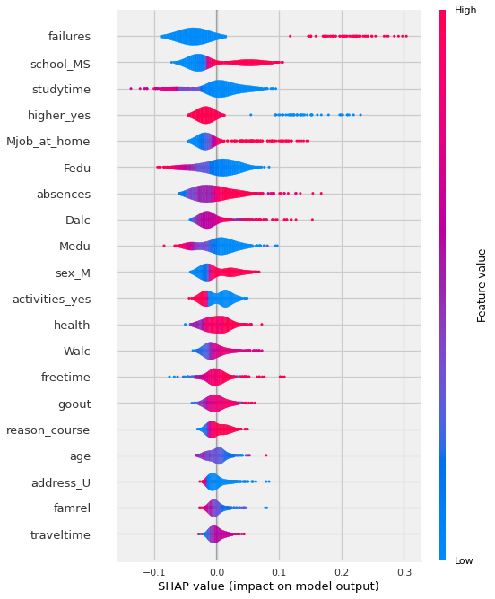
Summary Plot

## For normal bar graph of importance:
shap.summary_plot(shap_values[:,:,1],features=X_shap, plot_type='bar')

## For detail Shapely value visuals:
shap.summary_plot(shap_values[:,:,1], features=X_shap)

shap.summary_plot

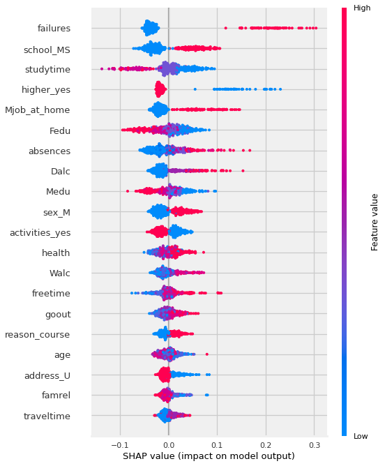
• Feature importance: Variables are ranked in descending order.

• Impact: The horizontal location shows whether the effect of that value is associated with a higher or lower prediction.

• Original value: Color shows whether that variable is high (in red) or low (in blue) for that observation.

• IMPORTANT NOTE: You may need to slice out the correct shap_values for the target class. (by default explainer.shap_values seems to return a list for a binary classification, one set of shap values for each class). - This will cause issues like the summary plot having a bar with an equal amount of blue and red for each class. - To fix, slice out the correct matrix from shap_values [0,1]

• First, let’s examine a simple version of our shap values.

  • By using the plot_type=”bar” version of the summary plot, we get something that looks very similar to the feature importances we discussed previously.

shap.summary_plot(shap_values[:,:,1],features= X_shap,plot_type='bar')

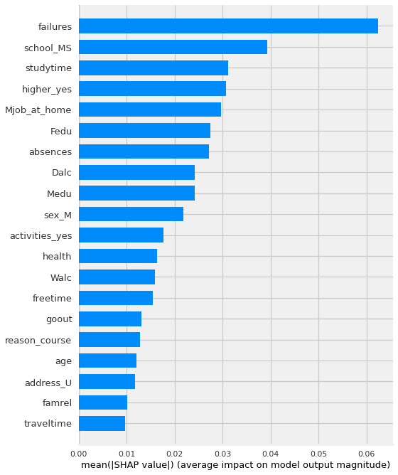
• In this case, it is using the magnitude of the average shap values to to show which features had the biggest impact on the model’s predictions.

  • Like feature importance and permutation importance, this visualization is not indicating which direction the features push the predict.

• Now, let’s examine the “dot” version of the summary plot.

  • By removing the plot_type argument, we are using the default, which is “dot”.

    • We could explicitly specify plot_type=”dot”.

      • There are also additional plot types that we will not be discussing in this lesson (e.g. “violin”,”compact_dot”)

# shap.summary_plot(shap_values[:,:,1],X_shap)

shap.summary_plot(shap_values[:,:,1],X_shap)

TO DO: “Failures””

Now THAT is a lot more nuanced of a visualization! Let’s break down how to interpret the visual above.

# shap.summary_plot(shap_values[:,:,1],features= X_shap,plot_type='compact_dot')

## violin version.
shap.summary_plot(shap_values[:,:,1],features= X_shap,plot_type='violin')

Dependence Plots

Shap also includes the shap.dependence_plot which show how the model output varies by a specific feature. By passing the function a feature name, it will automatically determine what features may driving the interactions with the selected feature. It will encode the interaction feature as color.

## To Auto-Select Feature Most correlated with a specific feature, just pass the desired feature's column name.

shap.dependence_plot('Age', shap_values[:,:,1], X_shap)

• TO DO:

  • There is a way to specifically call out multiple features but I wasn’t able to summarize it quickly for this nb

# shap_values[:,:,1].values

## Using shap_values made from shap_values = explainer(X_shap)
shap.dependence_plot("failures", shap_values[:,:,1].values,X_shap)

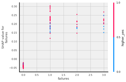
• ?Men are more likely to have failures?

## Using shap_values made from shap_values = explainer(X_shap)
shap.dependence_plot("sex_M", shap_values[:,:,1].values,X_shap)

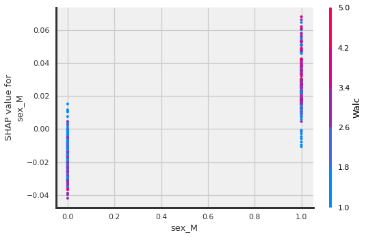
• ?Being male interacts with Weekend alcohol consumption??

## Using shap_values made from shap_values = explainer(X_shap)
shap.dependence_plot("age", shap_values[:,:,1].values,X_shap)

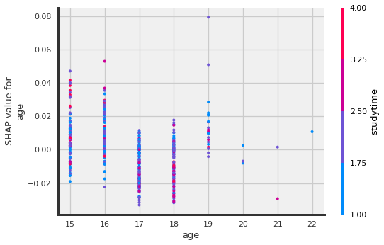
• ?The older the student the more likely the reason for this school was because of a specific course?

Force Plot

• Note: the force_plot is an interactive visualization that uses javascript. You must Trust your jupyter notebook in order to display it. - In the top right corner of jupyter notebook, next the kernel name (Python (dojo-env)), click the Not Trusted button to trust the notebook.

Global shap.force_plot

To show a global force plot:

## Fore plot
shap.force_plot(explainer.expected_value[1], shap_values[:,:,1], features=X_shap)

Global Force Plot

## TESTING COMPLEX SHAP VALS AGAIN (Overall Forceplot)
shap.force_plot(explainer.expected_value[1], shap_values[:,:,1].values,features=X_shap)

Visualization omitted, Javascript library not loaded!
Have you run `initjs()` in this notebook? If this notebook was from another user you must also trust this notebook (File -> Trust notebook). If you are viewing this notebook on github the Javascript has been stripped for security. If you are using JupyterLab this error is because a JupyterLab extension has not yet been written.

Fore Plot Interpretation

• TO DO

# ## Using explainer.shap_values for easier use of force plot
# shap_vals_simple = explainer.shap_values(X_shap)#,y_test)
# print(type(shap_vals_simple))
# shap_vals_simple[0].shape

# ## Overall Forceplot
# shap.force_plot(explainer.expected_value[1], shap_vals_simple[1],features=X_shap)

Explain Individual Plot

• To show an individual data point’s prediction and the factors pushing it towards one class or another.

• For now, we will randomly select a row to display, but we will revisit thoughtful selection of examples for stakeholders in our next lesson about local explanations.

## Just using np to randomly select a row
row = np.random.choice(range(len(X_shap)))         
shap.force_plot(explainer.expected_value[1], shap_values[1][row], X_shap.iloc[row])

row = np.random.choice(range(len(X_shap)))
print(f"- Row #: {row}")
print(f"- Target: {y_shap.iloc[row]}")
X_shap.iloc[row].round(2)

- Row #: 77
- Target: False

age                  16.0
Medu                  4.0
Fedu                  4.0
traveltime            1.0
studytime             1.0
failures              0.0
famrel                4.0
freetime              4.0
goout                 4.0
Dalc                  1.0
Walc                  2.0
health                2.0
absences              6.0
school_MS             0.0
sex_M                 0.0
address_U             1.0
famsize_LE3           0.0
Pstatus_T             1.0
Mjob_at_home          0.0
Mjob_health           1.0
Mjob_other            0.0
Mjob_services         0.0
Mjob_teacher          0.0
Fjob_at_home          0.0
Fjob_health           0.0
Fjob_other            1.0
Fjob_services         0.0
Fjob_teacher          0.0
reason_course         0.0
reason_home           1.0
reason_other          0.0
reason_reputation     0.0
guardian_father       0.0
guardian_mother       1.0
guardian_other        0.0
schoolsup_yes         0.0
famsup_yes            1.0
paid_yes              0.0
activities_yes        0.0
nursery_yes           1.0
higher_yes            1.0
internet_yes          1.0
romantic_yes          0.0
Name: 15, dtype: float64

# shap_vals_simple[1][row]

## Individual forceplot (with the complex shap vals)
shap.force_plot(explainer.expected_value[1],shap_values= shap_values[row,:,1].values,
               features=X_shap.iloc[row])

Visualization omitted, Javascript library not loaded!
Have you run `initjs()` in this notebook? If this notebook was from another user you must also trust this notebook (File -> Trust notebook). If you are viewing this notebook on github the Javascript has been stripped for security. If you are using JupyterLab this error is because a JupyterLab extension has not yet been written.

# ## Individual forceplot
# shap.force_plot(explainer.expected_value[1],shap_values= shap_vals_simple[1][row],
#                features=X_shap.iloc[row])

TEST: (move to next lesson)

from lime.lime_tabular import LimeTabularExplainer
lime_explainer =LimeTabularExplainer(
    training_data=np.array(X_shap),
    feature_names=X_shap.columns,
    class_names=['Died', 'Survived'],
    mode='classification'
)

exp = lime_explainer.explain_instance(X_shap.iloc[row], rf_clf.predict_proba)
exp.show_in_notebook(show_table=True)

X does not have valid feature names, but RandomForestClassifier was fitted with feature names

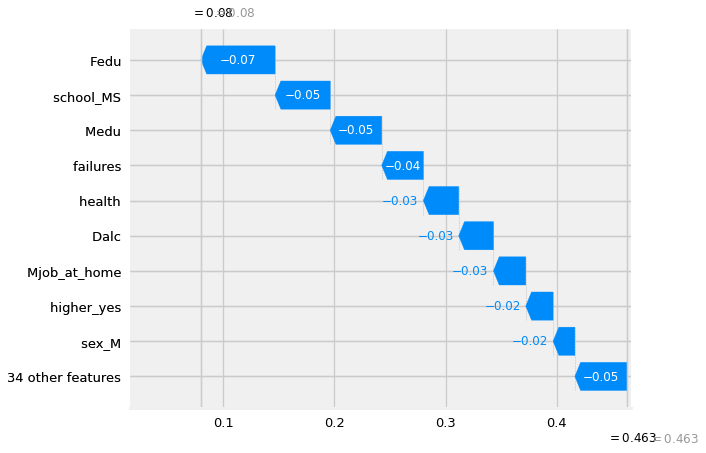
Waterfall Plot

explainer.expected_value

array([0.5367284, 0.4632716])

shap_values[row,:,1]

.values =
array([ 0.00435603, -0.046328  , -0.06670908, -0.00561117,  0.01695354,
       -0.03744232, -0.01199137, -0.0035424 ,  0.0071761 , -0.03123297,
       -0.01183418, -0.03183219,  0.0112064 , -0.04956995, -0.01958825,
       -0.01026708,  0.00046993,  0.0016435 , -0.02908411, -0.00373134,
        0.00057923, -0.00125725, -0.00077366, -0.00136103, -0.00273085,
       -0.00353734, -0.00186776,  0.00090522, -0.01188947, -0.01021466,
       -0.00110236,  0.00028077, -0.00193652,  0.00029861,  0.00066717,
       -0.00965465,  0.00079001, -0.00112643,  0.01878228, -0.00340502,
       -0.02457066, -0.00882573, -0.00436258])

.base_values =
0.4632716049382716

.data =
array([16.,  4.,  4.,  1.,  1.,  0.,  4.,  4.,  4.,  1.,  2.,  2.,  6.,
        0.,  0.,  1.,  0.,  1.,  0.,  1.,  0.,  0.,  0.,  0.,  0.,  1.,
        0.,  0.,  0.,  1.,  0.,  0.,  0.,  1.,  0.,  0.,  1.,  0.,  0.,
        1.,  1.,  1.,  0.])

#source: https://towardsdatascience.com/explainable-ai-xai-a-guide-to-7-packages-in-python-to-explain-your-models-932967f0634b
shap.plots._waterfall.waterfall_legacy(explainer.expected_value[1], 
                                       shap_values[row,:,1].values,
                                       features=X_shap.iloc[row],
                                       show=True)

Interaction Values

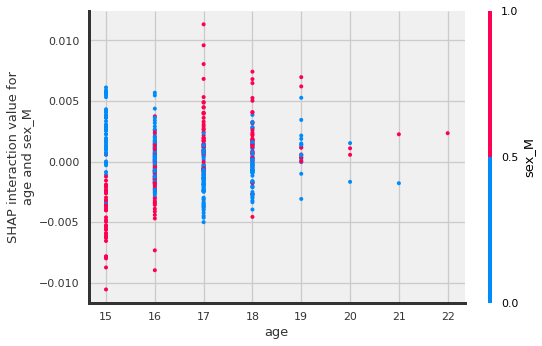
“The main effects are similar to the SHAP values you would get for a linear model, and the interaction effects captures all the higher-order interactions are divide them up among the pairwise interaction terms. Note that the sum of the entire interaction matrix is the difference between the model’s current output and expected output, and so the interaction effects on the off-diagonal are split in half (since there are two of each). When plotting interaction effects the SHAP package automatically multiplies the off-diagonal values by two to get the full interaction effect.”

• https://shap.readthedocs.io/en/latest/example_notebooks/tabular_examples/tree_based_models/NHANES I Survival Model.html#Compute-SHAP-Interaction-Values

• Interactions: - https://towardsdatascience.com/analysing-interactions-with-shap-8c4a2bc11c2a

shap_interaction_values = explainer.shap_interaction_values(X_shap)
shap.summary_plot(shap_interaction_values[0],X_shap)

shap.dependence_plot(
    ("age", "sex_M"),
    shap_interaction_values[1], X_shap,
    display_features=X_shap
)

shap.dependence_plot(
    ("goout", "Walc"),
    shap_interaction_values[1], X_shap,
    display_features=X_shap
)

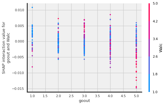
• The more the student goes out, the higher the Walc, and …(a negative shap interaction value would mean….🤔) BOOKMARK

TO DO: read more about the interactions and add interpretation here

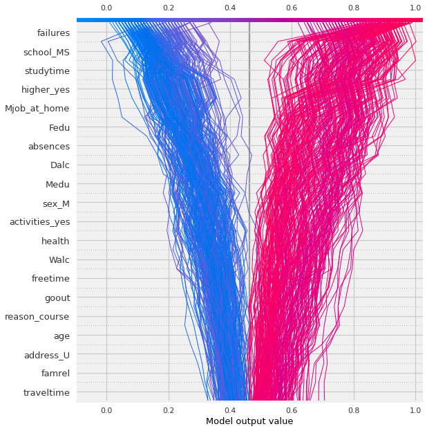
Shap Decision Plot?

• https://slundberg.github.io/shap/notebooks/plots/decision_plot.html

X_shap.loc[( X_shap['sex_M']==1) & (X_shap['Medu']>3) & (X_shap['goout']>2)\
          & (X_shap['reason_course']==1)]

	age	Medu	Fedu	traveltime	studytime	failures	famrel	freetime	goout	Dalc	Walc	health	absences	school_MS	sex_M	address_U	famsize_LE3	Pstatus_T	Mjob_at_home	Mjob_health	Mjob_other	Mjob_services	Mjob_teacher	Fjob_at_home	Fjob_health	Fjob_other	Fjob_services	Fjob_teacher	reason_course	reason_home	reason_other	reason_reputation	guardian_father	guardian_mother	guardian_other	schoolsup_yes	famsup_yes	paid_yes	activities_yes	nursery_yes	higher_yes	internet_yes	romantic_yes
13	15.0	4.0	3.0	2.0	2.0	0.0	5.0	4.0	3.0	1.0	2.0	3.0	0.0	0.0	1.0	1.0	0.0	1.0	0.0	0.0	0.0	0.0	1.0	0.0	0.0	1.0	0.0	0.0	1.0	0.0	0.0	0.0	0.0	1.0	0.0	0.0	1.0	0.0	0.0	1.0	1.0	1.0	0.0
42	15.0	4.0	4.0	1.0	2.0	0.0	4.0	3.0	3.0	1.0	1.0	5.0	0.0	0.0	1.0	1.0	0.0	1.0	0.0	0.0	0.0	1.0	0.0	0.0	0.0	0.0	0.0	1.0	1.0	0.0	0.0	0.0	1.0	0.0	0.0	0.0	1.0	0.0	1.0	1.0	1.0	1.0	0.0
71	15.0	4.0	2.0	1.0	4.0	0.0	3.0	3.0	3.0	1.0	1.0	3.0	0.0	0.0	1.0	1.0	0.0	1.0	0.0	0.0	1.0	0.0	0.0	0.0	0.0	1.0	0.0	0.0	1.0	0.0	0.0	0.0	0.0	1.0	0.0	0.0	0.0	0.0	0.0	1.0	1.0	1.0	0.0
128	16.0	4.0	4.0	1.0	1.0	0.0	3.0	5.0	5.0	2.0	5.0	4.0	8.0	0.0	1.0	0.0	0.0	1.0	0.0	0.0	0.0	0.0	1.0	0.0	0.0	0.0	0.0	1.0	1.0	0.0	0.0	0.0	0.0	1.0	0.0	0.0	0.0	0.0	1.0	1.0	1.0	1.0	0.0
193	17.0	4.0	3.0	1.0	2.0	0.0	5.0	2.0	3.0	1.0	1.0	2.0	4.0	0.0	1.0	1.0	0.0	1.0	0.0	0.0	1.0	0.0	0.0	0.0	0.0	1.0	0.0	0.0	1.0	0.0	0.0	0.0	0.0	1.0	0.0	0.0	1.0	1.0	1.0	1.0	1.0	1.0	1.0
102	15.0	4.0	4.0	1.0	1.0	0.0	5.0	3.0	3.0	1.0	1.0	5.0	2.0	0.0	1.0	1.0	0.0	1.0	0.0	0.0	0.0	1.0	0.0	0.0	0.0	1.0	0.0	0.0	1.0	0.0	0.0	0.0	0.0	1.0	0.0	0.0	1.0	1.0	1.0	0.0	1.0	1.0	0.0
268	17.0	4.0	4.0	2.0	2.0	0.0	3.0	3.0	3.0	2.0	3.0	4.0	0.0	0.0	1.0	0.0	1.0	0.0	0.0	0.0	0.0	0.0	1.0	0.0	0.0	1.0	0.0	0.0	1.0	0.0	0.0	0.0	0.0	1.0	0.0	0.0	1.0	0.0	0.0	1.0	1.0	1.0	0.0
267	17.0	4.0	3.0	2.0	2.0	0.0	2.0	5.0	5.0	1.0	4.0	5.0	8.0	0.0	1.0	1.0	1.0	1.0	0.0	1.0	0.0	0.0	0.0	0.0	0.0	1.0	0.0	0.0	1.0	0.0	0.0	0.0	0.0	1.0	0.0	0.0	0.0	0.0	1.0	1.0	1.0	1.0	1.0
543	17.0	4.0	4.0	3.0	1.0	3.0	3.0	3.0	3.0	1.0	3.0	5.0	2.0	1.0	1.0	0.0	0.0	1.0	0.0	1.0	0.0	0.0	0.0	0.0	0.0	1.0	0.0	0.0	1.0	0.0	0.0	0.0	1.0	0.0	0.0	0.0	0.0	0.0	1.0	1.0	1.0	1.0	1.0
501	16.0	4.0	3.0	1.0	1.0	0.0	4.0	2.0	5.0	1.0	5.0	5.0	8.0	1.0	1.0	1.0	1.0	1.0	0.0	0.0	1.0	0.0	0.0	0.0	0.0	1.0	0.0	0.0	1.0	0.0	0.0	0.0	1.0	0.0	0.0	0.0	0.0	0.0	1.0	1.0	1.0	1.0	0.0
361	19.0	4.0	2.0	2.0	2.0	0.0	5.0	4.0	4.0	1.0	1.0	1.0	9.0	0.0	1.0	1.0	0.0	1.0	0.0	1.0	0.0	0.0	0.0	0.0	0.0	1.0	0.0	0.0	1.0	0.0	0.0	0.0	0.0	1.0	0.0	0.0	1.0	0.0	1.0	1.0	1.0	1.0	1.0
76	15.0	4.0	0.0	2.0	4.0	0.0	3.0	4.0	3.0	1.0	1.0	1.0	0.0	0.0	1.0	1.0	0.0	1.0	0.0	0.0	0.0	0.0	1.0	0.0	0.0	1.0	0.0	0.0	1.0	0.0	0.0	0.0	0.0	1.0	0.0	0.0	0.0	0.0	1.0	1.0	1.0	1.0	0.0
12	15.0	4.0	4.0	1.0	1.0	0.0	4.0	3.0	3.0	1.0	3.0	5.0	0.0	0.0	1.0	1.0	1.0	1.0	0.0	1.0	0.0	0.0	0.0	0.0	0.0	0.0	1.0	0.0	1.0	0.0	0.0	0.0	1.0	0.0	0.0	0.0	1.0	0.0	1.0	1.0	1.0	1.0	0.0
189	17.0	4.0	3.0	2.0	2.0	0.0	4.0	4.0	4.0	4.0	4.0	4.0	0.0	0.0	1.0	1.0	1.0	1.0	0.0	0.0	0.0	0.0	1.0	0.0	0.0	1.0	0.0	0.0	1.0	0.0	0.0	0.0	0.0	1.0	0.0	0.0	0.0	0.0	1.0	1.0	1.0	1.0	0.0
401	18.0	4.0	3.0	1.0	3.0	0.0	5.0	4.0	5.0	2.0	3.0	5.0	0.0	0.0	1.0	1.0	0.0	1.0	0.0	0.0	0.0	0.0	1.0	0.0	0.0	1.0	0.0	0.0	1.0	0.0	0.0	0.0	0.0	1.0	0.0	0.0	1.0	0.0	0.0	1.0	1.0	1.0	1.0

X_shap['goout']

54     4.0
208    3.0
23     4.0
547    2.0
604    2.0
      ... 
410    4.0
168    4.0
401    5.0
124    4.0
538    3.0
Name: goout, Length: 486, dtype: float64

example = 13

shap.decision_plot(explainer.expected_value[1], shap_values[:,:,1].values,X_shap,
                  highlight=example)

📌 TO DO

• Try more targets.

  • Combine D and F into 1 group

  • Make a target about decrease in performance from g1 to g3.

APPENDIX

raise Exception('Do not include below in run all.')

---------------------------------------------------------------------------
Exception                                 Traceback (most recent call last)
Input In [58], in <cell line: 1>()
----> 1 raise Exception('Do not include below in run all.')

Exception: Do not include below in run all.

Lesson Creation Code

# [o for o in dir(shap) if 'Explainer' in o]

import pandas as pd
tables = pd.read_html("https://shap.readthedocs.io/en/latest/api.html")
len(tables)

explainers = tables[1]#.style.hide('index')
explainers.columns = ['Explainer','Description']
explainers['Explainer'] = explainers['Explainer'].map(lambda x: x.split('(')[0])
explainers

print(explainers.set_index("Explainer").to_markdown())