Model Explainers - For Regression#

Lesson Objectives#

By the end of this lesson students will be able to:

Define a global vs local explanation
Use the Shap package and interpret shap values.

Model Explainers#

There are packages with the sole purpose of better understanding how machine learning models make their predictions.
Generally, model explainers will take the model and some of your data and apply some iterative process to try to quantify how the features are influencing the model’s output.

import pandas as pd
import numpy as np
import matplotlib as mpl
import matplotlib.pyplot as plt
import seaborn as sns
## Customization Options
# pd.set_option('display.float_format',lambda x: f"{x:,.4f}")
pd.set_option("display.max_columns",100)
plt.style.use(['fivethirtyeight','seaborn-talk'])
mpl.rcParams['figure.facecolor']='white'

## additional required imports
from sklearn.model_selection import train_test_split
from sklearn.preprocessing import OneHotEncoder, StandardScaler
from sklearn.impute import SimpleImputer
from sklearn.compose import make_column_transformer, make_column_selector, ColumnTransformer
from sklearn.pipeline import make_pipeline, Pipeline
from sklearn import metrics

from sklearn.base import clone

## fixing random for lesson generation
SEED = 321
np.random.seed(SEED)

## Adding folder above to path
import os, sys
sys.path.append(os.path.abspath('../../'))

## Load stack_functions with autoreload turned on
%load_ext autoreload
%autoreload 2
from CODE import stack_functions as sf
from CODE import prisoner_project_functions as pf

def show_code(function):
    import inspect 
    from IPython.display import display,Markdown, display_markdown
    code = inspect.getsource(function)
    md_txt = f"```python\n{code}\n```"
    return display(Markdown(md_txt))
    

## Load in the student erformance data
url = "https://docs.google.com/spreadsheets/d/e/2PACX-1vS6xDKNpWkBBdhZSqepy48bXo55QnRv1Xy6tXTKYzZLMPjZozMfYhHQjAcC8uj9hQ/pub?output=xlsx"

df = pd.read_excel(url,sheet_name='student-mat')
# df.drop(columns=['G1','G2'])
df.info()
df.head()

<class 'pandas.core.frame.DataFrame'>
RangeIndex: 395 entries, 0 to 394
Data columns (total 33 columns):
 #   Column      Non-Null Count  Dtype  
---  ------      --------------  -----  
 school      395 non-null    object 
 sex         395 non-null    object 
 age         395 non-null    float64
 address     395 non-null    object 
 famsize     395 non-null    object 
 Pstatus     395 non-null    object 
 Medu        395 non-null    float64
 Fedu        395 non-null    float64
 Mjob        395 non-null    object 
 Fjob        395 non-null    object 
reason      395 non-null    object 
guardian    395 non-null    object 
traveltime  395 non-null    float64
studytime   395 non-null    float64
failures    395 non-null    float64
schoolsup   395 non-null    object 
famsup      395 non-null    object 
paid        395 non-null    object 
activities  395 non-null    object 
nursery     395 non-null    object 
higher      395 non-null    object 
internet    395 non-null    object 
romantic    395 non-null    object 
famrel      395 non-null    float64
freetime    395 non-null    float64
goout       395 non-null    float64
Dalc        395 non-null    float64
Walc        395 non-null    float64
health      395 non-null    float64
absences    395 non-null    float64
G1          395 non-null    float64
G2          395 non-null    float64
G3          395 non-null    float64
dtypes: float64(16), object(17)
memory usage: 102.0+ KB

	school	sex	age	address	famsize	Pstatus	Medu	Fedu	Mjob	Fjob	reason	guardian	traveltime	studytime	failures	schoolsup	famsup	paid	activities	nursery	higher	internet	romantic	famrel	freetime	goout	Dalc	Walc	health	absences	G1	G2	G3
0	GP	F	18.0	U	GT3	A	4.0	4.0	at_home	teacher	course	mother	2.0	2.0	0.0	yes	no	no	no	yes	yes	no	no	4.0	3.0	4.0	1.0	1.0	3.0	6.0	5.0	6.0	6.0
1	GP	F	17.0	U	GT3	T	1.0	1.0	at_home	other	course	father	1.0	2.0	0.0	no	yes	no	no	no	yes	yes	no	5.0	3.0	3.0	1.0	1.0	3.0	4.0	5.0	5.0	6.0
2	GP	F	15.0	U	LE3	T	1.0	1.0	at_home	other	other	mother	1.0	2.0	3.0	yes	no	yes	no	yes	yes	yes	no	4.0	3.0	2.0	2.0	3.0	3.0	10.0	7.0	8.0	10.0
3	GP	F	15.0	U	GT3	T	4.0	2.0	health	services	home	mother	1.0	3.0	0.0	no	yes	yes	yes	yes	yes	yes	yes	3.0	2.0	2.0	1.0	1.0	5.0	2.0	15.0	14.0	15.0
4	GP	F	16.0	U	GT3	T	3.0	3.0	other	other	home	father	1.0	2.0	0.0	no	yes	yes	no	yes	yes	no	no	4.0	3.0	2.0	1.0	2.0	5.0	4.0	6.0	10.0	10.0

# ### Train Test Split
## Make x and y variables
drop_feats = ['G1','G2']
y = df['G3'].copy()
X = df.drop(columns=['G3',*drop_feats]).copy()

## train-test-split with random state for reproducibility
X_train, X_test, y_train, y_test = train_test_split(X,y, random_state=SEED)


# ### Preprocessing + ColumnTransformer

## make categorical & numeric selectors
cat_sel = make_column_selector(dtype_include='object')
num_sel = make_column_selector(dtype_include='number')

## make pipelines for categorical vs numeric data
cat_pipe = make_pipeline(SimpleImputer(strategy='constant',
                                       fill_value='MISSING'),
                         OneHotEncoder(drop='if_binary', sparse=False))

num_pipe = make_pipeline(SimpleImputer(strategy='mean'))

## make the preprocessing column transformer
preprocessor = make_column_transformer((num_pipe, num_sel),
                                       (cat_pipe,cat_sel),
                                      verbose_feature_names_out=False)

## fit column transformer and run get_feature_names_out
preprocessor.fit(X_train)
feature_names = preprocessor.get_feature_names_out()

X_train_df = pd.DataFrame(preprocessor.transform(X_train), 
                          columns = feature_names, index = X_train.index)


X_test_df = pd.DataFrame(preprocessor.transform(X_test), 
                          columns = feature_names, index = X_test.index)
X_test_df.head(3)

	age	Medu	Fedu	traveltime	studytime	famrel	freetime	goout	Dalc	Walc	health	absences	sex_M	address_U	famsize_LE3	Pstatus_T	Mjob_health	Mjob_other	Mjob_services	Fjob_at_home	Fjob_services	reason_home	reason_reputation	guardian_father	guardian_mother	schoolsup_yes	famsup_yes	paid_yes	activities_yes	nursery_yes	higher_yes	internet_yes
58	15.0	1.0	2.0	1.0	2.0	4.0	3.0	2.0	1.0	1.0	5.0	2.0	1.0	1.0	1.0	1.0	0.0	1.0	0.0	1.0	0.0	1.0	0.0	1.0	0.0	1.0	1.0	0.0	1.0	1.0	1.0	1.0
338	18.0	3.0	3.0	1.0	4.0	5.0	3.0	3.0	1.0	1.0	1.0	7.0	0.0	1.0	1.0	1.0	0.0	0.0	1.0	0.0	1.0	1.0	0.0	0.0	1.0	0.0	1.0	0.0	0.0	1.0	1.0	1.0
291	17.0	4.0	3.0	1.0	3.0	4.0	2.0	2.0	1.0	2.0	3.0	0.0	0.0	1.0	0.0	1.0	1.0	0.0	0.0	0.0	1.0	0.0	1.0	0.0	1.0	0.0	1.0	1.0	0.0	1.0	1.0	1.0

## fit random fores
from sklearn.ensemble import RandomForestRegressor
rf_reg = RandomForestRegressor()
rf_reg.fit(X_train_df,y_train)
sf.evaluate_regression(rf_reg,X_test_df,y_test, warn=False,
                       X_train=X_train_df, y_train=y_train)#linreg(rf_reg,X_train_zips,y_train,X_test_zips,y_test)

      Train   Test  Delta
R^2   0.910  0.085 -0.825
RMSE  1.405  4.023  2.618

Fjob_health          0.001351
guardian_mother      0.004300
reason_other         0.004932
guardian_father      0.005284
reason_home          0.005356
internet_yes         0.005659
Pstatus_T            0.006196
paid_yes             0.007169
address_U            0.007630
Mjob_health          0.007761
Mjob_other           0.007970
famsize_LE3          0.008351
Fjob_services        0.008621
Mjob_teacher         0.009024
Dalc                 0.009191
school_MS            0.009252
nursery_yes          0.009272
Fjob_other           0.009453
Mjob_services        0.010012
activities_yes       0.010288
Fjob_teacher         0.010371
guardian_other       0.010720
Fjob_at_home         0.010922
romantic_yes         0.012431
famsup_yes           0.013015
higher_yes           0.014331
reason_reputation    0.015734
Fedu                 0.020560
sex_M                0.021505
famrel               0.021921
reason_course        0.022823
Mjob_at_home         0.023137
schoolsup_yes        0.023192
Medu                 0.024457
age                  0.027299
traveltime           0.027808
health               0.031356
freetime             0.035128
Walc                 0.036055
studytime            0.038027
goout                0.047714
failures             0.151020
absences             0.213404
Name: Feature Importance, dtype: float64

Loading Joblib of Regressions from Lesson 04#

import joblib
## If showing joblib in prior lesson, this cell will be included and further explained
loaded_data = joblib.load("../3_Feature_Importance/lesson_03.joblib")
loaded_data.keys()

dict_keys(['X_train', 'y_train', 'X_test', 'y_test', 'preprocessor', 'lin_reg', 'rf_reg'])

## If showing joblib in prior lesson, this cell will be included and further explained
X_train_reg = loaded_data['X_train'].copy()
y_train_reg = loaded_data['y_train'].copy()
X_test_df_reg = loaded_data['X_test'].copy()
y_test_reg = loaded_data['y_test'].copy()
lin_reg = loaded_data['lin_reg']
rf_reg = loaded_data['rf_reg']

Using SHAP for Model Interpretation#

SHAP (SHapley Additive exPlanations))
- Repository
- Documentation
SHAP uses game theory to calcualte Shapely values for each feature in the dataset.
Shapely values are calculated by iteratively testing each feature’s contribution to the model by comparing the model’s performance with vs. without the feature. (The “marginal contribution” of the feature to the model’s performance).

Papers, Book Excerpts, and Blogs#

White Paper on Shapely Values
Intepretable Machine Learning Book - Section on SHAP
Towards Data Science Blog Posts:
- Explain Your Model with SHAP Values
- Explain Any Model with SHAP KernelExplaibner

Videos/Talks:#

Explaining Machine Learning Models (in general).
- “Open the Black Box: an intro to Model Interpretability with LIME and SHAP
Understanding Shapely/SHAP Values:
- AI Simplified: SHAP Values in Machine Learning - (Intuitive Explanation)
- Explainable AI explained! | #4 SHAP - (Math Calculation Explanation)

How To Use Shap#

Import and initialize javascript:

import shap 
shap.initjs()

import shap
shap.initjs()

Shap Explainers#

shap has several types of model explainers that are optimized for different types of models.

Explainers and their use cases:#

Explainer	Description
shap.Explainer	Uses Shapley values to explain any machine learning model or python function.
shap.explainers.Tree	Uses Tree SHAP algorithms to explain the output of ensemble tree models.
shap.explainers.Linear	Computes SHAP values for a linear model, optionally accounting for inter-feature correlations.
shap.explainers.Permutation	This method approximates the Shapley values by iterating through permutations of the inputs.

See this blog post for intro to topic and how to use with trees
For non-tree/random forest models see this follow up post

Preparing Data for Shap#

Shap’s approach to explaining models can be very resource-intensive for complex models such as our RandomForest.
To get around this issue, shap includes a convenient smapling function to save a small sample from one of our X variables.

X_shap = shap.sample(X_train_df,nsamples=200,random_state=321)
X_shap

	age	Medu	Fedu	traveltime	studytime	failures	famrel	freetime	goout	Dalc	Walc	health	absences	school_MS	sex_M	address_U	famsize_LE3	Pstatus_T	Mjob_at_home	Mjob_health	Mjob_other	Mjob_services	Mjob_teacher	Fjob_at_home	Fjob_health	Fjob_other	Fjob_services	Fjob_teacher	reason_course	reason_home	reason_other	reason_reputation	guardian_father	guardian_mother	guardian_other	schoolsup_yes	famsup_yes	paid_yes	activities_yes	nursery_yes	higher_yes	internet_yes	romantic_yes
355	18.0	3.0	3.0	1.0	2.0	0.0	5.0	3.0	4.0	1.0	1.0	5.0	0.0	1.0	0.0	1.0	0.0	1.0	0.0	0.0	0.0	1.0	0.0	0.0	0.0	0.0	1.0	0.0	1.0	0.0	0.0	0.0	1.0	0.0	0.0	0.0	1.0	0.0	0.0	1.0	1.0	0.0	1.0
354	17.0	4.0	3.0	2.0	2.0	0.0	4.0	5.0	5.0	1.0	3.0	2.0	4.0	1.0	1.0	0.0	0.0	1.0	0.0	0.0	0.0	1.0	0.0	0.0	0.0	1.0	0.0	0.0	0.0	1.0	0.0	0.0	0.0	1.0	0.0	0.0	1.0	1.0	1.0	0.0	1.0	1.0	1.0
328	17.0	4.0	4.0	1.0	3.0	0.0	5.0	4.0	4.0	1.0	3.0	4.0	7.0	0.0	0.0	1.0	0.0	1.0	0.0	0.0	0.0	0.0	1.0	0.0	0.0	0.0	1.0	0.0	1.0	0.0	0.0	0.0	0.0	1.0	0.0	0.0	1.0	1.0	1.0	1.0	1.0	1.0	0.0
231	17.0	2.0	2.0	2.0	2.0	0.0	4.0	5.0	2.0	1.0	1.0	1.0	4.0	0.0	1.0	0.0	0.0	1.0	0.0	0.0	1.0	0.0	0.0	0.0	0.0	1.0	0.0	0.0	1.0	0.0	0.0	0.0	1.0	0.0	0.0	0.0	1.0	1.0	1.0	1.0	1.0	1.0	0.0
312	19.0	1.0	2.0	1.0	2.0	1.0	4.0	5.0	2.0	2.0	2.0	4.0	3.0	0.0	1.0	1.0	0.0	1.0	0.0	0.0	1.0	0.0	0.0	0.0	0.0	0.0	1.0	0.0	1.0	0.0	0.0	0.0	0.0	0.0	1.0	0.0	0.0	0.0	0.0	0.0	1.0	1.0	0.0
...	...	...	...	...	...	...	...	...	...	...	...	...	...	...	...	...	...	...	...	...	...	...	...	...	...	...	...	...	...	...	...	...	...	...	...	...	...	...	...	...	...	...	...
210	19.0	3.0	3.0	1.0	4.0	0.0	4.0	3.0	3.0	1.0	2.0	3.0	10.0	0.0	0.0	1.0	0.0	1.0	0.0	0.0	1.0	0.0	0.0	0.0	0.0	1.0	0.0	0.0	0.0	0.0	0.0	1.0	0.0	0.0	1.0	0.0	1.0	1.0	1.0	1.0	1.0	1.0	0.0
236	17.0	2.0	2.0	1.0	2.0	0.0	4.0	4.0	2.0	5.0	5.0	4.0	4.0	0.0	1.0	1.0	1.0	1.0	0.0	0.0	1.0	0.0	0.0	0.0	0.0	1.0	0.0	0.0	0.0	1.0	0.0	0.0	1.0	0.0	0.0	0.0	0.0	1.0	1.0	0.0	1.0	1.0	1.0
10	15.0	4.0	4.0	1.0	2.0	0.0	3.0	3.0	3.0	1.0	2.0	2.0	0.0	0.0	0.0	1.0	0.0	1.0	0.0	0.0	0.0	0.0	1.0	0.0	1.0	0.0	0.0	0.0	0.0	0.0	0.0	1.0	0.0	1.0	0.0	0.0	1.0	1.0	0.0	1.0	1.0	1.0	0.0
13	15.0	4.0	3.0	2.0	2.0	0.0	5.0	4.0	3.0	1.0	2.0	3.0	2.0	0.0	1.0	1.0	0.0	1.0	0.0	0.0	0.0	0.0	1.0	0.0	0.0	1.0	0.0	0.0	1.0	0.0	0.0	0.0	0.0	1.0	0.0	0.0	1.0	1.0	0.0	1.0	1.0	1.0	0.0
372	17.0	2.0	2.0	1.0	3.0	0.0	3.0	4.0	3.0	1.0	1.0	3.0	8.0	1.0	0.0	1.0	0.0	1.0	0.0	0.0	1.0	0.0	0.0	1.0	0.0	0.0	0.0	0.0	0.0	1.0	0.0	0.0	0.0	1.0	0.0	0.0	0.0	0.0	1.0	1.0	1.0	0.0	1.0

200 rows × 43 columns

## get the corresponding y-values
y_shap = y_train.loc[X_shap.index]
y_shap

   9.0
  11.0
   9.0
  11.0
  11.0
       ... 
   8.0
  13.0
    9.0
   11.0
  11.0
Name: G3, Length: 200, dtype: float64

Explaining Our RandomForest#

Create a shap explainer using your fit model.

explainer = shap.TreeExplainer(rf_reg)

Get shapely values from explainer for your training data

shap_values = explainer(X_shap)

Select which type of the available plots you’d like to visualize

Types of Plots:
- summary_plot()
- dependence_plot()
- force_plot() for a given observation
- force_plot() for all data

X_shap = X_train_df.copy()#shap.sample(X_train_df,nsamples=200,random_state=SEED)

explainer = shap.TreeExplainer(rf_reg)
shap_values = explainer(X_shap,y_shap)
shap_values[0]

.values =
array([-2.65129202e-03,  3.37739374e-02, -1.66913694e-02,  4.04224947e-02,
       -8.89278699e-02,  8.22963912e-01, -2.19713066e-02,  9.46616336e-03,
       -1.05073602e-01,  4.45105221e-02,  7.95999848e-02,  6.99744889e-01,
        1.05407076e+00,  7.37235898e-03, -1.65178625e-01,  1.09019192e-01,
        6.88803146e-02, -8.73117299e-03,  1.44210492e-01, -4.05021571e-02,
        8.44343694e-03, -5.94057998e-02,  9.03834608e-02,  2.51376396e-02,
        1.69540791e-03, -5.10195738e-02, -2.51987310e-03, -3.91344713e-02,
        1.97009755e-01, -3.56228354e-03, -2.04581060e-02,  2.76732166e-01,
       -1.81765629e-03,  1.43730639e-02,  5.16251179e-02,  1.98845113e-01,
        2.61826118e-01, -5.57521403e-04, -2.41598627e-02,  3.22229694e-02,
        9.33188335e-03,  3.45140981e-02,  7.30116122e-02])

.base_values =
array([10.34317568])

.data =
array([17.,  3.,  2.,  2.,  2.,  0.,  4.,  4.,  4.,  1.,  3.,  1.,  2.,
        0.,  0.,  1.,  1.,  1.,  0.,  0.,  1.,  0.,  0.,  0.,  0.,  1.,
        0.,  0.,  0.,  0.,  0.,  1.,  0.,  1.,  0.,  0.,  0.,  1.,  0.,
        1.,  1.,  1.,  0.])

X_shap.shape

(296, 43)

shap_values.shape

(296, 43)

We can see that shap calculated values for every row/column in our X_shap variable.
What does the first row’s shap values look like?

shap_values[0]

.values =
array([-2.65129202e-03,  3.37739374e-02, -1.66913694e-02,  4.04224947e-02,
       -8.89278699e-02,  8.22963912e-01, -2.19713066e-02,  9.46616336e-03,
       -1.05073602e-01,  4.45105221e-02,  7.95999848e-02,  6.99744889e-01,
        1.05407076e+00,  7.37235898e-03, -1.65178625e-01,  1.09019192e-01,
        6.88803146e-02, -8.73117299e-03,  1.44210492e-01, -4.05021571e-02,
        8.44343694e-03, -5.94057998e-02,  9.03834608e-02,  2.51376396e-02,
        1.69540791e-03, -5.10195738e-02, -2.51987310e-03, -3.91344713e-02,
        1.97009755e-01, -3.56228354e-03, -2.04581060e-02,  2.76732166e-01,
       -1.81765629e-03,  1.43730639e-02,  5.16251179e-02,  1.98845113e-01,
        2.61826118e-01, -5.57521403e-04, -2.41598627e-02,  3.22229694e-02,
        9.33188335e-03,  3.45140981e-02,  7.30116122e-02])

.base_values =
array([10.34317568])

.data =
array([17.,  3.,  2.,  2.,  2.,  0.,  4.,  4.,  4.,  1.,  3.,  1.,  2.,
        0.,  0.,  1.,  1.,  1.,  0.,  0.,  1.,  0.,  0.,  0.,  0.,  1.,
        0.,  0.,  0.,  0.,  0.,  1.,  0.,  1.,  0.,  0.,  0.,  1.,  0.,
        1.,  1.,  1.,  0.])

Notice above that we do not seem to have a simple numpy array.

type(shap_values[0])

shap._explanation.Explanation

explanation_0 = shap_values[0]
explanation_0

.values =
array([-2.65129202e-03,  3.37739374e-02, -1.66913694e-02,  4.04224947e-02,
       -8.89278699e-02,  8.22963912e-01, -2.19713066e-02,  9.46616336e-03,
       -1.05073602e-01,  4.45105221e-02,  7.95999848e-02,  6.99744889e-01,
        1.05407076e+00,  7.37235898e-03, -1.65178625e-01,  1.09019192e-01,
        6.88803146e-02, -8.73117299e-03,  1.44210492e-01, -4.05021571e-02,
        8.44343694e-03, -5.94057998e-02,  9.03834608e-02,  2.51376396e-02,
        1.69540791e-03, -5.10195738e-02, -2.51987310e-03, -3.91344713e-02,
        1.97009755e-01, -3.56228354e-03, -2.04581060e-02,  2.76732166e-01,
       -1.81765629e-03,  1.43730639e-02,  5.16251179e-02,  1.98845113e-01,
        2.61826118e-01, -5.57521403e-04, -2.41598627e-02,  3.22229694e-02,
        9.33188335e-03,  3.45140981e-02,  7.30116122e-02])

.base_values =
array([10.34317568])

.data =
array([17.,  3.,  2.,  2.,  2.,  0.,  4.,  4.,  4.,  1.,  3.,  1.,  2.,
        0.,  0.,  1.,  1.,  1.,  0.,  0.,  1.,  0.,  0.,  0.,  0.,  1.,
        0.,  0.,  0.,  0.,  0.,  1.,  0.,  1.,  0.,  0.,  0.,  1.,  0.,
        1.,  1.,  1.,  0.])

Each entry in the shap_values array is new type of object called an Explanation.
- Each Explanation has:
  - values:the shap values calculated for this observation/row.
    - For classification models, there is a column with values for each target.
  - base_values: the final shap output value
  - data: the original input feature

## Showing .data is the same as the raw X_shap
explanation_0.data

array([17.,  3.,  2.,  2.,  2.,  0.,  4.,  4.,  4.,  1.,  3.,  1.,  2.,
        0.,  0.,  1.,  1.,  1.,  0.,  0.,  1.,  0.,  0.,  0.,  0.,  1.,
        0.,  0.,  0.,  0.,  0.,  1.,  0.,  1.,  0.,  0.,  0.,  1.,  0.,
        1.,  1.,  1.,  0.])

X_shap.iloc[0].values

array([17.,  3.,  2.,  2.,  2.,  0.,  4.,  4.,  4.,  1.,  3.,  1.,  2.,
        0.,  0.,  1.,  1.,  1.,  0.,  0.,  1.,  0.,  0.,  0.,  0.,  1.,
        0.,  0.,  0.,  0.,  0.,  1.,  0.,  1.,  0.,  0.,  0.,  1.,  0.,
        1.,  1.,  1.,  0.])

## showing the .values
pd.Series(explanation_0.values,index=X_shap.columns)

age                 -0.002651
Medu                 0.033774
Fedu                -0.016691
traveltime           0.040422
studytime           -0.088928
failures             0.822964
famrel              -0.021971
freetime             0.009466
goout               -0.105074
Dalc                 0.044511
Walc                 0.079600
health               0.699745
absences             1.054071
school_MS            0.007372
sex_M               -0.165179
address_U            0.109019
famsize_LE3          0.068880
Pstatus_T           -0.008731
Mjob_at_home         0.144210
Mjob_health         -0.040502
Mjob_other           0.008443
Mjob_services       -0.059406
Mjob_teacher         0.090383
Fjob_at_home         0.025138
Fjob_health          0.001695
Fjob_other          -0.051020
Fjob_services       -0.002520
Fjob_teacher        -0.039134
reason_course        0.197010
reason_home         -0.003562
reason_other        -0.020458
reason_reputation    0.276732
guardian_father     -0.001818
guardian_mother      0.014373
guardian_other       0.051625
schoolsup_yes        0.198845
famsup_yes           0.261826
paid_yes            -0.000558
activities_yes      -0.024160
nursery_yes          0.032223
higher_yes           0.009332
internet_yes         0.034514
romantic_yes         0.073012
dtype: float64

Shap Visualizations - Regression#

Summary Plot#

## For normal bar graph of importance:
shap.summary_plot(shap_values, features=X_shap, plot_type='bar')

## For detail Shapely value visuals:
shap.summary_plot(shap_values, features=X_shap)

shap.summary_plot

Feature importance: Variables are ranked in descending order.

Impact: The horizontal location shows whether the effect of that value is associated with a higher or lower prediction.
Original value: Color shows whether that variable is high (in red) or low (in blue) for that observation.

IMPORTANT NOTE: You may need to slice out the correct shap_values for the target class. (by default explainer.shap_values seems to return a list for a binary classification, one set of shap values for each class). - This will cause issues like the summary plot having a bar with an equal amount of blue and red for each class. - To fix, slice out the correct matrix from shap_values [0,1]

First, let’s examine a simple version of our shap values.
- By using the plot_type=”bar” version of the summary plot, we get something that looks very similar to the feature importances we discussed previously.

shap.summary_plot(shap_values,features= X_shap,plot_type='bar')

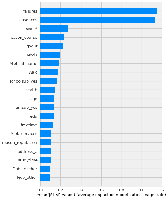
../../_images/4_Model_Explainers-Regression_44_0.png

In this case, it is using the magnitude of the average shap values to to show which features had the biggest impact on the model’s predictions.
- Like feature importance and permutation importance, this visualization is not indicating which direction the features push the predict.
Now, let’s examine the “dot” version of the summary plot.
- By removing the plot_type argument, we are using the default, which is “dot”.
  - We could explicitly specify plot_type=”dot”.
    - There are also additional plot types that we will not be discussing in this lesson (e.g. “violin”,”compact_dot”)

shap.summary_plot(shap_values,X_shap)

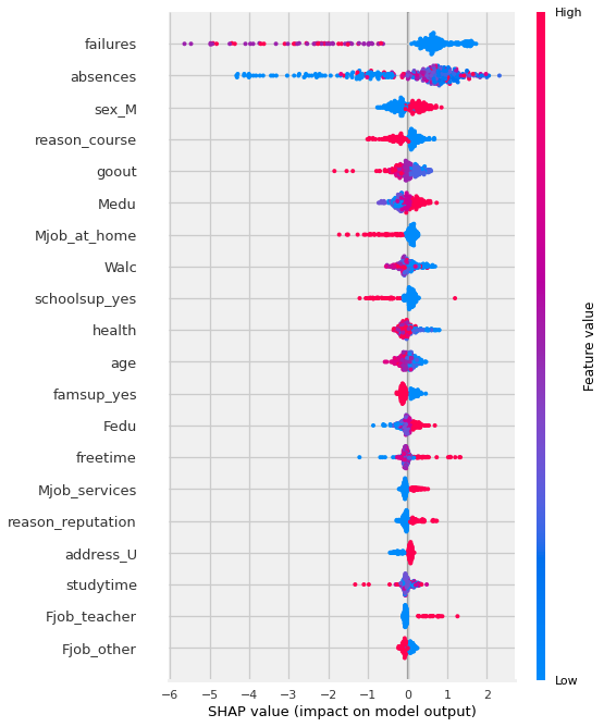
../../_images/4_Model_Explainers-Regression_46_0.png

Now THAT is a lot more nuanced of a visualization! Let’s break down how to interpret the visual above.

Reading Summary Plots#

In the summary plot above:
- Each dot represents an observation/row (in this case, a student).
- The features are plotting on the y-axis, and are sorted from the most impactful features to the least (from top to bottom).
- The calculated Shapely values for each observation are plotted on the x-axis. The most positive the value the more positive… bookmark
- For each feature, the original values of that feature are represented with color.
  - Using the default colormap, blue represents the lowest value in the column and red represents the highest.
    - For one hot encoded categories, blue=0, red = 1.
    - For numeric features: the shade of the color indicates where it falls in the feature’s distribution.

Summary Plot Interpretation#

fewer prior failures = higher final grade -Q: what is going on with absences?
- why are some of the lowest values leading to negative shap value (meaning a decreased final score)?
- Why would less absences meaning a lower final grade?
  - 🤔 Did the student not spend all 3 years at the school??
sex_M:
- males get a higher grade
reason_course:
- if a student attends the school because of a specific course, they have a lower final grade.
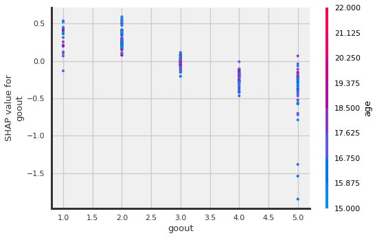
goout:
- the more a student goes out, the lower the grade.
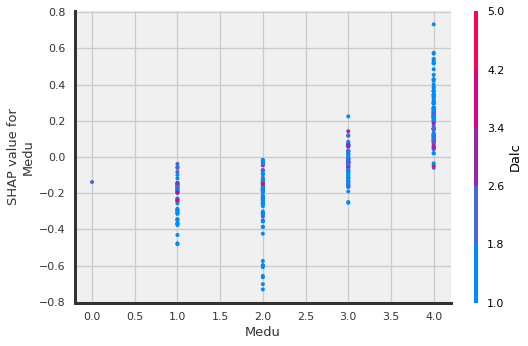
Medu (mother’s education):
- Higher mother’s ed the higher the grade
Mjob_at_home:
- Mother at home leads to lower grades.
Walc: Lower weekend alcohol consumption “causes” higher grade

Dependence Plots#

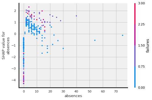
Shap also includes the shap.dependence_plot which show how the model output varies by a specific feature. By passing the function a feature name, it will automatically determine what features may driving the interactions with the selected feature. It will encode the interaction feature as color.

## To Auto-Select Feature Most correlated with a specific feature, just pass the desired feature's column name.

shap.dependence_plot('age', shap_values, X_shap)

TO DO:
- There is a way to specifically call out multiple features but I wasn’t able to summarize it quickly for this nb

## Using shap_values made from shap_values = explainer(X_shap)
shap.dependence_plot("absences", shap_values.values,X_shap)

../../_images/4_Model_Explainers-Regression_53_0.png

## Using shap_values made from shap_values = explainer(X_shap)
shap.dependence_plot("Medu", shap_values.values,X_shap)

../../_images/4_Model_Explainers-Regression_54_0.png

## Using shap_values made from shap_values = explainer(X_shap)
shap.dependence_plot("goout", shap_values.values,X_shap)

../../_images/4_Model_Explainers-Regression_55_0.png

Force Plot#

Note: the force_plot is an interactive visualization that uses javascript. You must Trust your jupyter notebook in order to display it. - In the top right corner of jupyter notebook, next the kernel name (Python (dojo-env)), click the Not Trusted button to trust the notebook.

Global `shap.force_plot`#

To show a global force plot:

## Fore plot
shap.force_plot(explainer.expected_value[1], shap_values[:,:,1], features=X_shap)

Global Force Plot#

## TESTING COMPLEX SHAP VALS AGAIN (Overall Forceplot)
shap.force_plot(explainer.expected_value, shap_values.values,features=X_shap)

Visualization omitted, Javascript library not loaded!
Have you run `initjs()` in this notebook? If this notebook was from another user you must also trust this notebook (File -> Trust notebook). If you are viewing this notebook on github the Javascript has been stripped for security. If you are using JupyterLab this error is because a JupyterLab extension has not yet been written.

Fore Plot Interpretation#

TO DO

Explain Individual Plot#

To show an individual data point’s prediction and the factors pushing it towards one class or another.
For now, we will randomly select a row to display, but we will revisit thoughtful selection of examples for stakeholders in our next lesson about local explanations.

## Just using np to randomly select a row
row = np.random.choice(range(len(X_shap)))         
shap.force_plot(explainer.expected_value[1], shap_values[1][row], X_shap.iloc[row])

row = np.random.choice(range(len(X_shap)))
print(f"- Row #: {row}")
print(f"- Target: {y_shap.iloc[row]}")
X_shap.iloc[row].round(2)

- Row #: 85
- Target: 6.0

age                  18.0
Medu                  1.0
Fedu                  1.0
traveltime            2.0
studytime             2.0
failures              1.0
famrel                4.0
freetime              4.0
goout                 3.0
Dalc                  2.0
Walc                  3.0
health                5.0
absences              2.0
school_MS             1.0
sex_M                 1.0
address_U             0.0
famsize_LE3           1.0
Pstatus_T             1.0
Mjob_at_home          1.0
Mjob_health           0.0
Mjob_other            0.0
Mjob_services         0.0
Mjob_teacher          0.0
Fjob_at_home          0.0
Fjob_health           0.0
Fjob_other            1.0
Fjob_services         0.0
Fjob_teacher          0.0
reason_course         0.0
reason_home           0.0
reason_other          1.0
reason_reputation     0.0
guardian_father       0.0
guardian_mother       1.0
guardian_other        0.0
schoolsup_yes         0.0
famsup_yes            0.0
paid_yes              0.0
activities_yes        1.0
nursery_yes           0.0
higher_yes            0.0
internet_yes          0.0
romantic_yes          0.0
Name: 361, dtype: float64

## Individual forceplot (with the complex shap vals)
shap.force_plot(explainer.expected_value,shap_values= shap_values[row].values,
               features=X_shap.iloc[row])

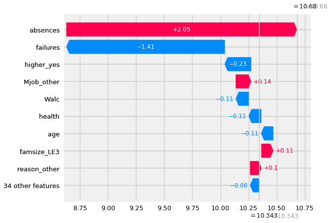
Waterfall Plot#

explainer.expected_value

array([10.34317568])

shap_values[row]#,:,1]

.values =
array([-1.06826576e-01, -8.27475108e-02, -9.09468180e-02, -1.41339274e-02,
       -5.23458955e-02, -1.40791878e+00,  6.95681721e-03, -4.14373232e-02,
       -7.43381448e-02, -3.20156255e-02, -1.14419829e-01, -1.11251761e-01,
        2.04968238e+00,  2.65195333e-02,  4.74230874e-02, -8.60920840e-02,
        1.05248311e-01, -7.51729126e-03,  7.89352552e-02, -1.64113732e-02,
        1.35993462e-01, -2.18647657e-02,  1.99391968e-02, -1.90337616e-02,
       -1.55896265e-03, -3.25649041e-02,  2.07980786e-03, -2.77867960e-02,
        9.32572748e-02,  1.00607556e-02,  1.00138176e-01, -1.92533952e-02,
        3.49964031e-03, -4.32813322e-03, -1.97932944e-04,  3.07952569e-02,
        9.92020595e-02, -8.22436248e-03,  6.61156139e-02, -1.49940694e-02,
       -2.34602883e-01,  4.27374105e-02,  4.10531897e-02])

.base_values =
array([10.34317568])

.data =
array([18.,  1.,  1.,  2.,  2.,  1.,  4.,  4.,  3.,  2.,  3.,  5.,  2.,
        1.,  1.,  0.,  1.,  1.,  1.,  0.,  0.,  0.,  0.,  0.,  0.,  1.,
        0.,  0.,  0.,  0.,  1.,  0.,  0.,  1.,  0.,  0.,  0.,  0.,  1.,
        0.,  0.,  0.,  0.])

#source: https://towardsdatascience.com/explainable-ai-xai-a-guide-to-7-packages-in-python-to-explain-your-models-932967f0634b
shap.plots._waterfall.waterfall_legacy(explainer.expected_value[0], 
                                       shap_values[row].values,
                                       features=X_shap.iloc[row],
                                       show=True)

../../_images/4_Model_Explainers-Regression_71_0.png

BOOKMARK: stopped here 07/11/22#

Interaction Values#

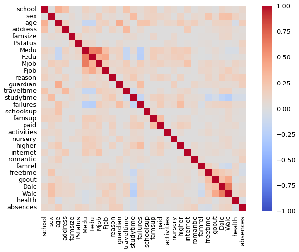
“The main effects are similar to the SHAP values you would get for a linear model, and the interaction effects captures all the higher-order interactions are divide them up among the pairwise interaction terms. Note that the sum of the entire interaction matrix is the difference between the model’s current output and expected output, and so the interaction effects on the off-diagonal are split in half (since there are two of each). When plotting interaction effects the SHAP package automatically multiplies the off-diagonal values by two to get the full interaction effect.”

https://shap.readthedocs.io/en/latest/example_notebooks/tabular_examples/tree_based_models/NHANES I Survival Model.html#Compute-SHAP-Interaction-Values

from dython.nominal import associations
res = associations(X, annot=False,cmap='coolwarm')
len(res)

../../_images/4_Model_Explainers-Regression_75_0.png

Interactions: - https://towardsdatascience.com/analysing-interactions-with-shap-8c4a2bc11c2a

shap_interaction_values = explainer.shap_interaction_values(X_shap)
shap.summary_plot(shap_interaction_values,X_shap)

shap.dependence_plot(
    ("age", "Walc"),
    shap_interaction_values, X_shap,
    display_features=X_shap
)

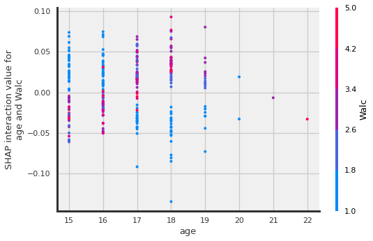
../../_images/4_Model_Explainers-Regression_78_0.png

TO DO: read more about the interactions and add interpretation here

`Shap Decision Plot?`#

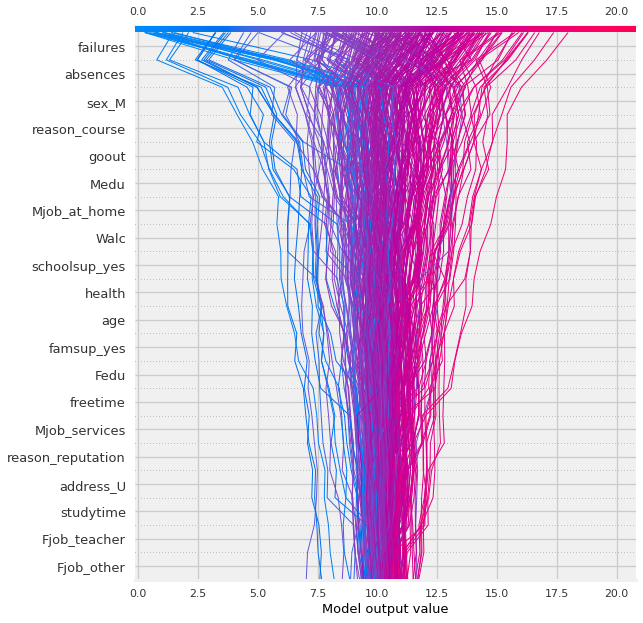
shap.decision_plot(explainer.expected_value, shap_values.values,X_shap)

../../_images/4_Model_Explainers-Regression_81_0.png

Stack 5: Data Visualization - Model Insights

Model Explainers - For Regression

Contents

Model Explainers - For Regression#

Lesson Objectives#

Model Explainers#

Loading Joblib of Regressions from Lesson 04#

Using SHAP for Model Interpretation#

Papers, Book Excerpts, and Blogs#

Videos/Talks:#

How To Use Shap#

Shap Explainers#

Explainers and their use cases:#

Preparing Data for Shap#

Explaining Our RandomForest#

Shap Visualizations - Regression#

Summary Plot#

Reading Summary Plots#

Summary Plot Interpretation#

Dependence Plots#

Force Plot#

Global `shap.force_plot`#

Global Force Plot#

Fore Plot Interpretation#

Explain Individual Plot#

Waterfall Plot#

BOOKMARK: stopped here 07/11/22#

Interaction Values#

`Shap Decision Plot?`#

Stack 5: Data Visualization - Model Insights

Model Explainers - For Regression

Contents

Model Explainers - For Regression#

Lesson Objectives#

Model Explainers#

Loading Joblib of Regressions from Lesson 04#

Using SHAP for Model Interpretation#

Papers, Book Excerpts, and Blogs#

Videos/Talks:#

How To Use Shap#

Shap Explainers#

Explainers and their use cases:#

Preparing Data for Shap#

Explaining Our RandomForest#

Shap Visualizations - Regression#

Summary Plot#

Reading Summary Plots#

Summary Plot Interpretation#

Dependence Plots#

Force Plot#

Global shap.force_plot#

Global Force Plot#

Fore Plot Interpretation#

Explain Individual Plot#

Waterfall Plot#

BOOKMARK: stopped here 07/11/22#

Interaction Values#

Shap Decision Plot?#

Global `shap.force_plot`#

`Shap Decision Plot?`#